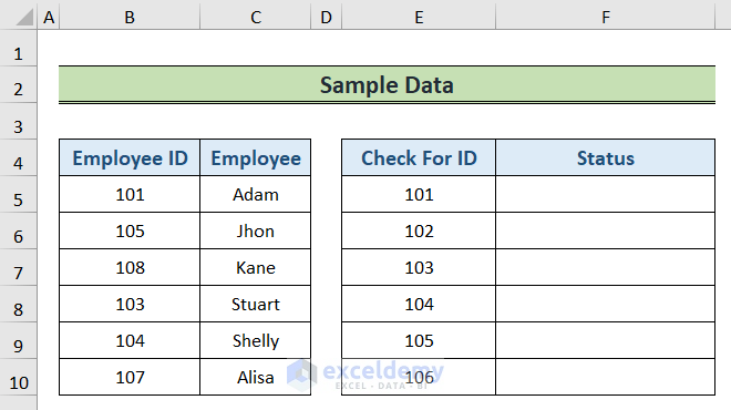
Let’s use the following sample dataset to illustrate the methods for checking missing values.
Method 1 – Using Combination of IF and COUNTIF Functions
Steps:
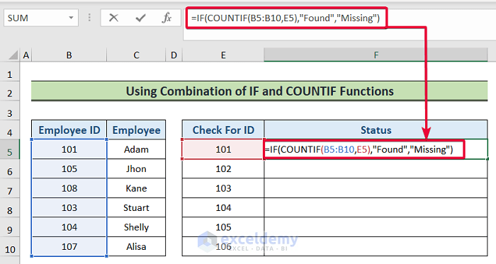
- Select the F5 cell and write the following formula:
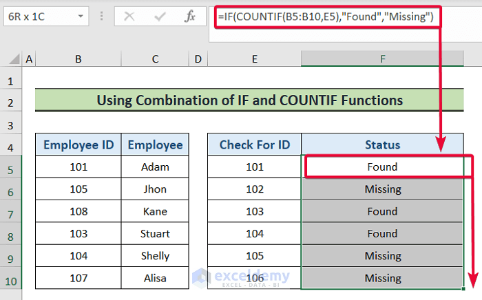
=IF(COUNTIF(B5:B10,E5),"Found","Missing")- Hit Enter.
- You will find the values that are missing from the Employee ID list.
Formula Breakdown:
- COUNTIF(B5:B10,E5): The COUNTIF function counts the number of cells that satisfy a specified criterion. It returns zero if no cells satisfy the requirement. In this case, the function will go through the range (B5:B10) and look for the value in the E5 If it finds it, then it will return 1. Otherwise, it will return zero.
- IF(COUNTIF(B5:B10,E5),”Found”,”Missing”): Any non-zero value will be treated as TRUE by the IF function, and zero will be treated as FALSE. In the formula, the COUNTIF function will either return zero or one. If it returns zero, the IF function will treat it as FALSE and will return “Missing”, the second output. And if the COUNTIF function returns one, then the IF function will return “Found”. In this particular case, the COUNTIF function will return 1, and thus the IF function will return “Found”.
Read More: How to Fill Missing Values in Excel
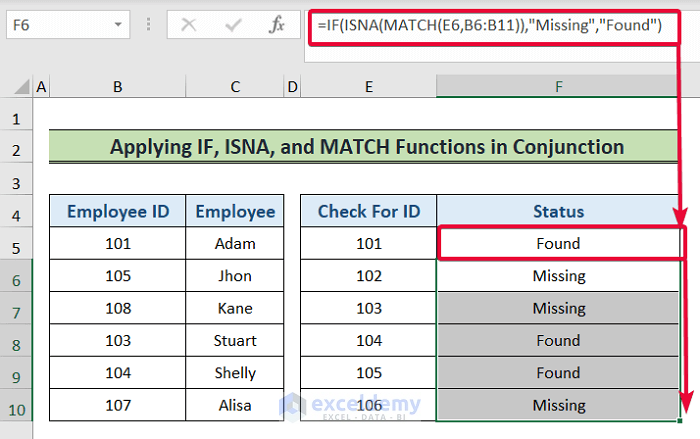
Method 2 – Combining IF, ISNA, and MATCH Functions
Steps:
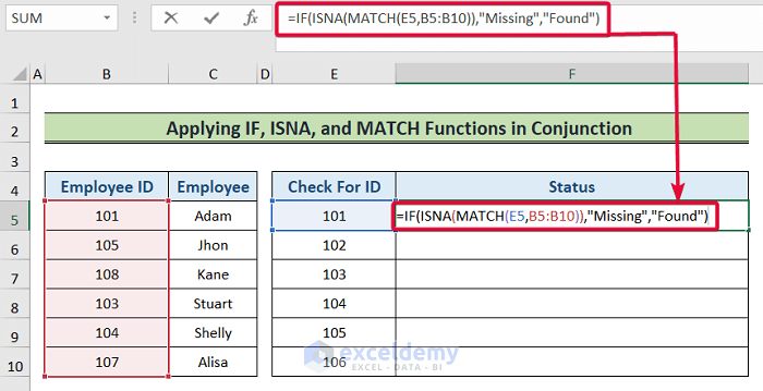
- Choose cell F5 and enter the following formula:
=IF(ISNA(MATCH(E5,B5:B10)),"Missing","Found")- Press Enter.
- You will discover the missing values from the Employee IDcolumn.
Formula Breakdown:
- MATCH(E5,B5:B10): The MATCH function goes through a range looking for a particular value. If it finds the value, then it returns the position of the value in numeric value. In this case, the MATCH function will find a match in the range (B5:B10) for the value in the E5 cell and will return a numeric value as its position in the range.
- ISNA(MATCH(E5,B5:B10)): The ISNA function returns TRUE if a formula returns the #N/A error value; otherwise, it returns FALSE. Here, the MATCH function will return a numeric value and so the ISNA function will assign FALSE to that value.
- IF(ISNA(MATCH(E5,B5:B10)),”Missing”,”Found”): The IF function evaluates the first argument. If the argument is TRUE then it returns the second argument and if not, it returns the third argument. Here, the ISNA function will return FALSE and so the IF function will return “Found”. This means the value is present in the (B5:B10)
Read More: How to Filter Missing Data in Excel
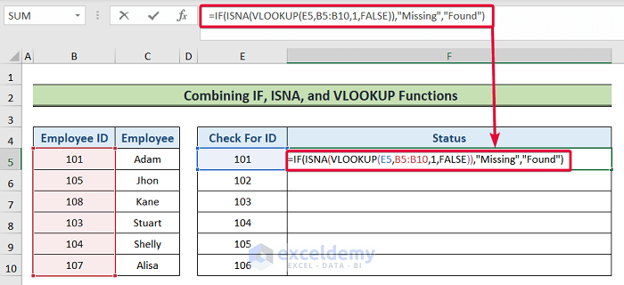
Method 3 – Applying IF, ISNA, and VLOOKUP Functions in Conjunction
Steps:
- Choose cell F5 and enter the following formula:
=IF(ISNA(VLOOKUP(E5,B5:B10,1,FALSE)),"Missing","Found")- Press the Enter button.
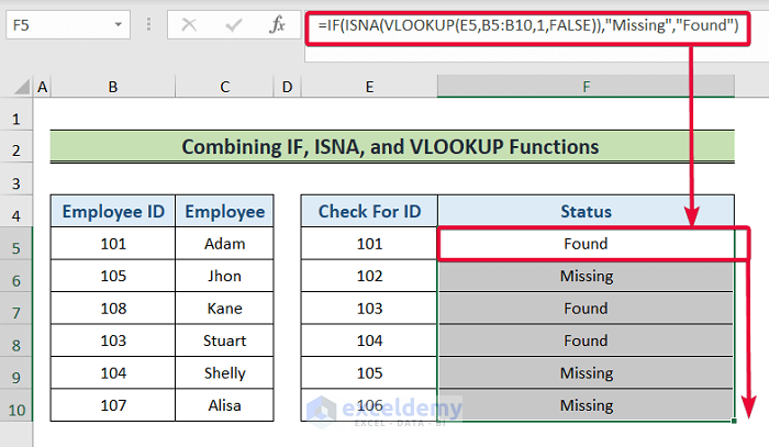
- You will see what values are missing from the Employee ID column.
Formula Breakdown:
- VLOOKUP(E5,B5:B10,1,FALSE): Here, the VLOOKUP function will look for the value in the E5 cell in the (B5:B10) If it finds the value, then it will return 1, otherwise, it will return FALSE.
- ISNA(VLOOKUP(E5,B5:B10,1,FALSE)): The ISNA function returns TRUE if a formula returns the #N/A error value; otherwise, it returns FALSE. Here, the VLOOKUP function will return 1 and so the ISNA function will assign FALSE to that value.
- IF(ISNA(MATCH(E5,B5:B10)),”Missing”,”Found”): The initial argument is assessed by the IF function. If the argument is TRUE then it returns the second argument, and if not, it returns the third argument. Here, the ISNA function will return FALSE, and so the IF function will return “Found”. This means the value is present in the (B5:B10)
Read More: How to Deal with Missing Data in Excel
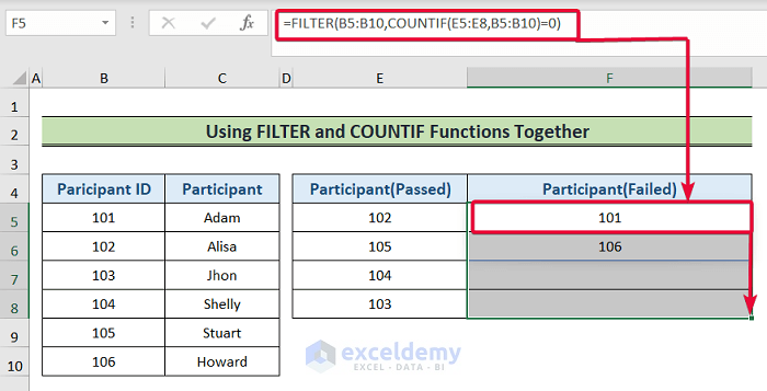
Using FILTER and COUNTIF Functions Together to Compare Two Lists for Missing Values
FILTER is available on Excel 2019 and newer, as well as Excel for Microsoft 365.
Steps:
- Choose cell F5 and enter the formula below:
=FILTER(B5:B10,COUNTIF(E5:E8,B5:B10)=0)- Hit Enter.
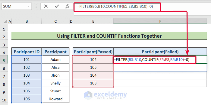
- You will see which participant IDs are missing from the previous column.
Formula Breakdown:
- COUNTIF(E5:E8,B5:B10): Here, the COUNTIF function will count the number of each value in the present in the range (E5:E8). The criteria for counting are the values in the range (B5:B10). For example, it will look for the value 102 in the (E5:E8I range as the value is present in the (B5:B10) r If it finds the value, then it counts as one. If it finds the value multiple times, then it will assign the number of times it has counted the value. On the other hand, if it does not find the value, then it will count as zero. In this case, the value 101 is not present in the (E5:E8) range, thus it will count as zero.
- FILTER(B5:B10,COUNTIF(E5:E8,B5:B10)=0): The FILTER function will filter out the values from the range B5:B10 that the COUNTIF function will count zero times. In this way, the formula will find the missing values in the Participant (passed) list that is present in the Participant.
Read More: How to Compare Two Excel Sheets to Find Missing Data
Download Practice Workbook
Related Articles
- How to Cross Reference in Excel to Find Missing Data
- How to Remove Missing Values in Excel
- How to Find Missing Rows in Excel
- How to Count Missing Values in Excel
<< Go Back To Missing Values in Excel | Data Cleaning in Excel | Learn Excel
Get FREE Advanced Excel Exercises with Solutions!
