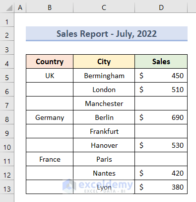
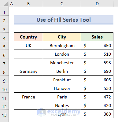
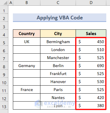
The sample dataset shows the information of sales amount of some cities in 3 different countries. We will fill some blank values.
Method 1 – Use the Fill Series Tool to Fill Missing Values
- Select the cell range D6:D8.
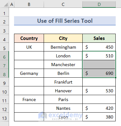
- Go to the Home tab and click on the Fill icon under the Editing group.

- Select Series from the drop-down menu.

- The Series window will appear.
- Select Columns and Growth under the Series in and Type sections, respectively.
- Mark the Trend box.
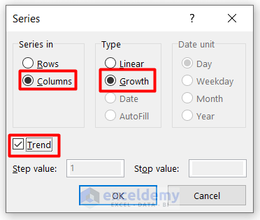
- Press OK. You’ll get the values that would fill the series between these two end-points.
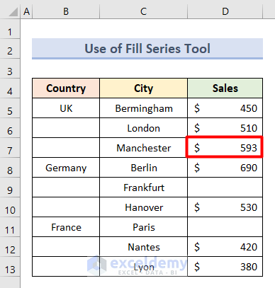
- Follow the similar process to get the other numerical values.
Read More: How to Deal with Missing Data in Excel
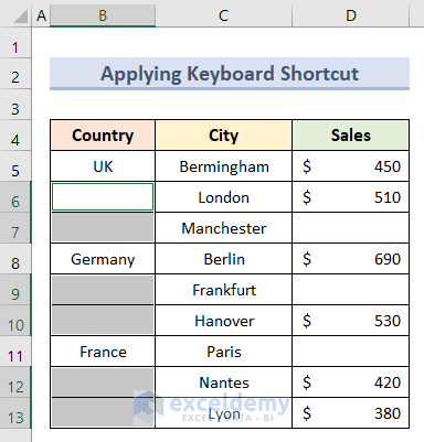
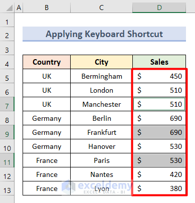
Method 2 – Fill Missing Values in Excel with a Keyboard Shortcut
- Select the first blank value in the column you want to fill.
- Press the Ctrl + Down key on your keyboard to select all the blank cells at once.
- Insert this formula in cell B6.
=B5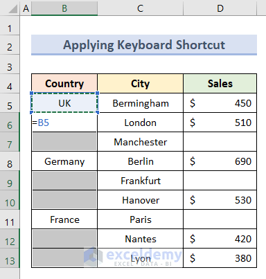
We used cell B5 as the reference cell for the selected blank cells. Therefore, cell B6 will get value from cell B5.
- Press Ctrl + Enter.
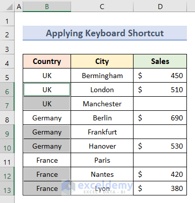
- Copy column B and paste it back into itself as Values.

Read More: How to Find Missing Values in Excel
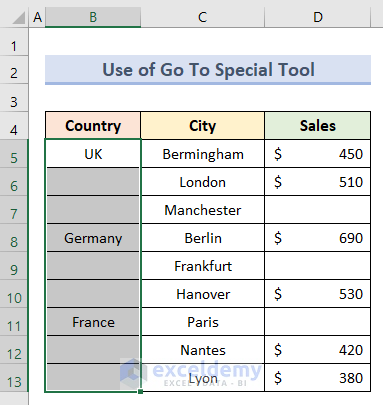
Method 3 – Use the Go To Special Tool to Fill Missing Values
- Select the cell range B5:B13.
- Go to the Home tab and click on Find & Select.
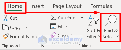
- Select Go To Special from the drop-down section.

- You will see the Go To Special window.
- Select Blanks and hit OK.
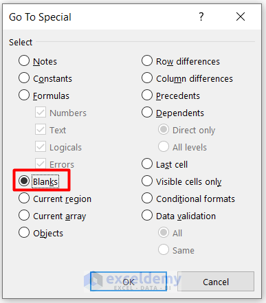
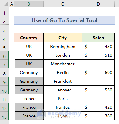
- The blank cells will be separated.
- Insert this formula in cell B6.
=B5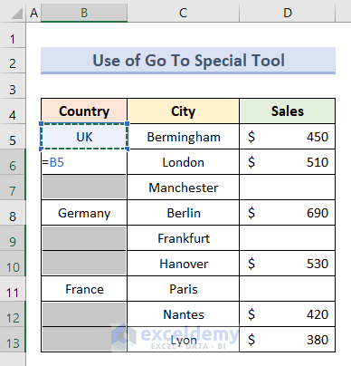
- Press Ctrl + Enter.
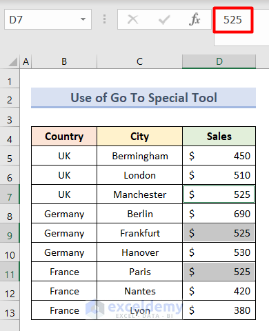
- For repetitive numeric values, select the blank cells as described above.
- Insert your desired value on the formula bar.
- Press Ctrl + Enter and you will see the final output.
Method 4 – Fill Missing Values with Excel VBA Code
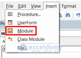
- Go to the Developer tab and select Visual Basic.

- Click on Module under the Insert tab.
- Insert this code in the blank page.
Sub Fill_blank_cells_with_missing_value()
Dim wk As Worksheet
Dim rg As Range
Set wk = Worksheets("VBA")
For Each rg In wk.Range("D5:D13")
If IsEmpty(rg) Then
rg.Value = 525
End If
Next
End Sub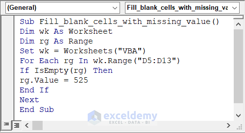
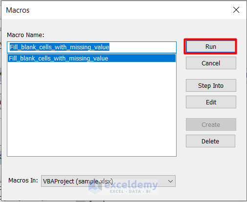
- Click on the Run Sub button or press F5 on your keyboard.

- Press Run on the Macros window.
- You can see the missing values in the dataset.
Read More: How to Filter Missing Data in Excel
Method 5 – Apply the INDEX Function to Interpolate Missing Values in Excel
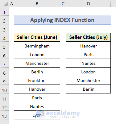
- We prepared two lists of seller cities based on the month of June and July. The second list has some missing city names.
- Insert this formula in cell D11.
=INDEX($B$5:$B$13,MATCH(TRUE,ISNA(MATCH($B$5:$B$13,$D$5:D10,0)),0))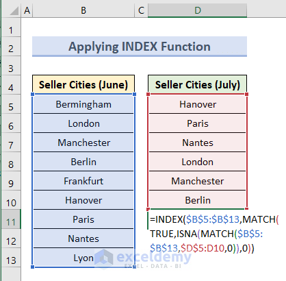
We used the INDEX function to compare the selected cells. Then, we applied the MATCH function to search for the specified missing value with the condition TRUE. Lastly, we applied the ISNA function to avoid an error with a 0 in the end for getting an exact match.
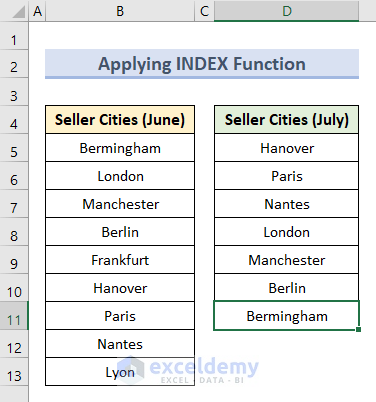
- Press Shift + Ctrl + Enter.
- We have our first missing value.
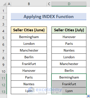
- Drag the bottom corner of cell D11 to cell D13 to get the final output.
Download the Practice Workbook
Related Articles
- How to Find Missing Rows in Excel
- How to Count Missing Values in Excel
- Compare Two Excel Sheets to Find Missing Data
- How to Cross Reference in Excel to Find Missing Data
- How to Remove Missing Values in Excel
<< Go Back To Missing Values in Excel | Data Cleaning in Excel | Learn Excel
Get FREE Advanced Excel Exercises with Solutions!
