Today we will learn how to find missing values in a list in Excel. We may sometimes find ourselves searching for certain values in a list in our daily lives. To tackle those situations, read this article carefully.
How to Find Missing Values in a List in Excel: 3 Useful Methods
In this section, we will demonstrate 3 effective methods to find missing values in a list in Excel. To display the methods, we have created an example where a list of the top 10 goal scorers in a tournament is given. And on the right side, there are some names of the players. Now we want to find out if the given names on the right sides are actually on the list of top 10 goal scorers or not.

So let’s begin with our first method.
1. Combine IF and COUNTIF Functions to Find Missing Values
Steps:
Here we have combined the IF and COUNTIF functions and used the following formula in cell E5.
=IF(COUNTIF(B5:B14,D5),"Yes","Missing")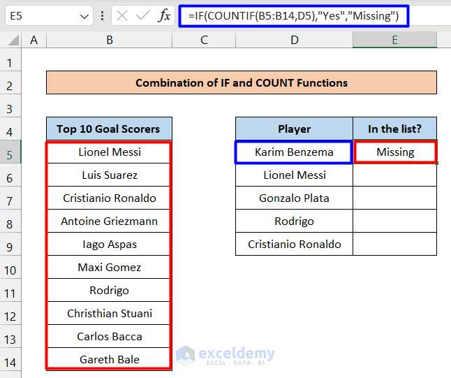
Where,
- B5:B14 is the cell range of the list where the name will be searched.
- D5 is the name of the player to be searched.
- “Yes” is the result shown when the player is found in the list.
- “No” is the result shown when the player is not found in the list.
To use the same formula for cells from E6 to E9, use the following steps.
- Bring your mouse cursor to B5 in the formula bar and click the f4 You will see that the dollar sign “$” has appeared before B and 5.
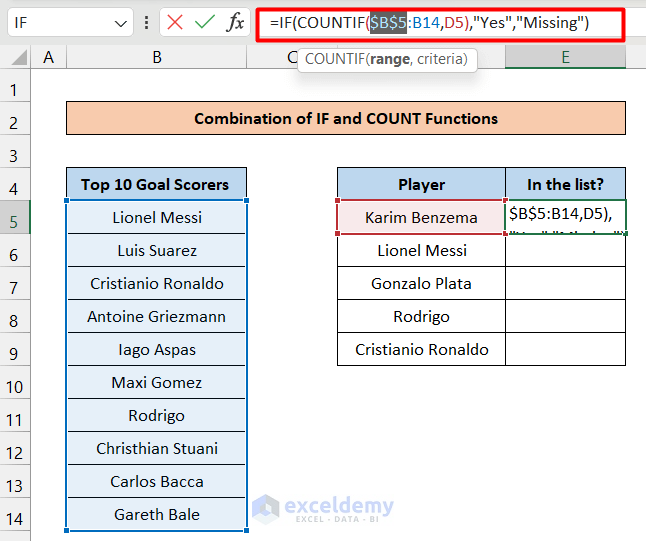
- Now do the same thing for B14. As a result, you should get the same result as this below.

- Now bring your mouse cursor to the bottom right corner of cell E5. You should notice a sign like “+”.

- Now drag it down to E9. You should get the results like this.

Read More: How to Deal with Missing Data in Excel
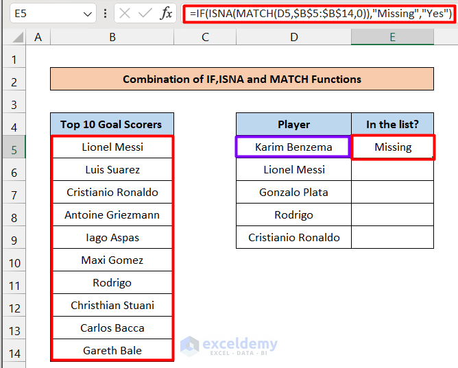
2. Merge IF, ISNA, and MATCH Functions to Find Missing Values
Steps:
- In this method, we will use the MATCH and ISNA functions along with the IF function. The formula is below:
=IF(ISNA(MATCH(D5,B5:B14,0)),”Missing”,”Yes”)
=IF(ISNA(MATCH(D5,B5:B14,0)),"Missing","Yes")Here,
- D5 is the player to be searched in the list.
- B5:B14 is the range of the list.
- 0 is for Exact matching.
- “Missing” will be the result if the condition is true.
- “Yes” will be the result if the condition is false.
- Now, following the method described in method 1, you can apply a similar formula for other cells and get the same result.

Read More: How to Filter Missing Data in Excel
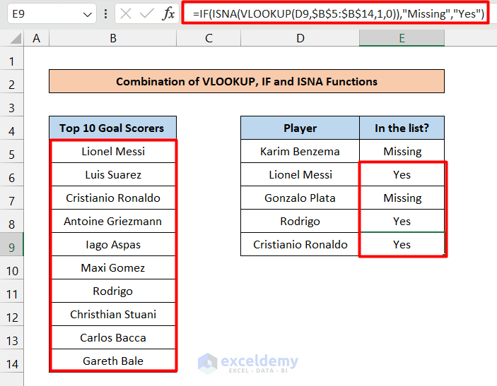
3. Combine IF, ISNA, and VLOOKUP Functions to Find Missing Values
Steps:
- We can also use the VLOOKUP function instead of the MATCH function to accomplish our task of finding missing values in a list in Excel. So the formula will be like this:
=IF(ISNA(VLOOKUP(D9,B5:B14,1,0)),"Missing","Yes")Where
- D5 is the player to be searched in the list.
- B5:B14 is the range of the list.
- 1 is the column number in the array(range) where the player will be searched.
- 0 is for Exact matching.
- “Missing” will be the result if the condition is true.
- “Yes” will be the result if the condition is false.
The result will be similar to the previous one.

- Now apply the formula to the cells below, and you will get the result like this.
Read More: How to Fill Missing Values in Excel
Things to Remember
- Use the 1st method for simplicity.
- Use the 2nd and 3rd methods if you want to apply more advanced Excel functions.
Download Practice Workbook
Download this practice workbook to exercise while you are reading this article.
Conclusion
Hope you enjoyed this article about how to find missing values in a list in Excel. Please comment in the post if you have any further queries.
Related Articles
- How to Find Missing Rows in Excel
- How to Cross Reference in Excel to Find Missing Data
- How to Compare Two Excel Sheets to Find Missing Data
- How to Count Missing Values in Excel
- How to Remove Missing Values in Excel
<< Go Back To Missing Values in Excel | Data Cleaning in Excel | Learn Excel
Get FREE Advanced Excel Exercises with Solutions!
