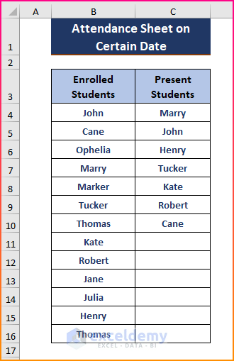
We have two columns that hold student names and want to find the missing entries among the columns by using cross-referencing.
How to Cross Reference in Excel to Find Missing Data: 6 Easy Ways
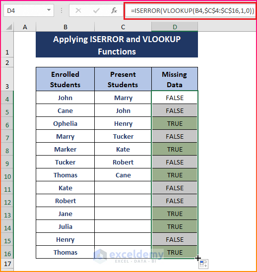
Method 1 – Applying ISERROR and VLOOKUP Functions to Identify Missing Data
Steps:
- Insert the following formula in cell D4.
=ISERROR(VLOOKUP(B4,$C$4:$C$16,1,0))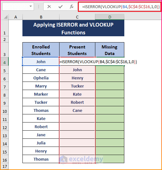
Formula Explanation
- The VLOOKUP function takes B4 as lookup_value, $C$4:$C$16 as table_array, 1 as col_index_num, and 0 as [range_lookup].
- Whenever VLOOKUP yields in #N/A Error, the ISERROR function puts TRUE or FALSE in places where error occurs or not respectively.
- Press Enter to apply the inserted formula, then drag the Fill Handle to execute the formula for other cells.
Read More: How to Deal with Missing Data in Excel
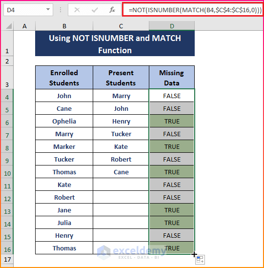
Method 2 – Cross Referencing Data Using NOT, ISNUMBER, and MATCH Functions
Steps:
- Paste the following formula in the D4 cell.
=NOT(ISNUMBER(MATCH(B4,$C$4:$C$16,0)))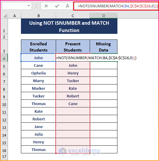
Formula Explanation
- The MATCH function returns 2 as the lookup_values (i.e., B4) found in row 2 within the lookup_array (i.e., $C$4:$C$16).
- After that, the ISNUMBER function returns TRUE or FALSE depending on the MATCH outcomes. Finally, the NOT function turns the Trues into Falses or vice versa.
- Use the Enter key to execute the formula.
- Drag the Fill Handle to apply the formula to the other cells.
Read More: How to Find Missing Values in Excel
Method 3 – Fetching Missing Data Using IF, ISERROR, and VLOOKUP Functions in Excel
Steps:
- Insert the following formula in D4.
=IF(ISERROR(VLOOKUP(B4,$C$4:$C$16,1,FALSE)),B4, "")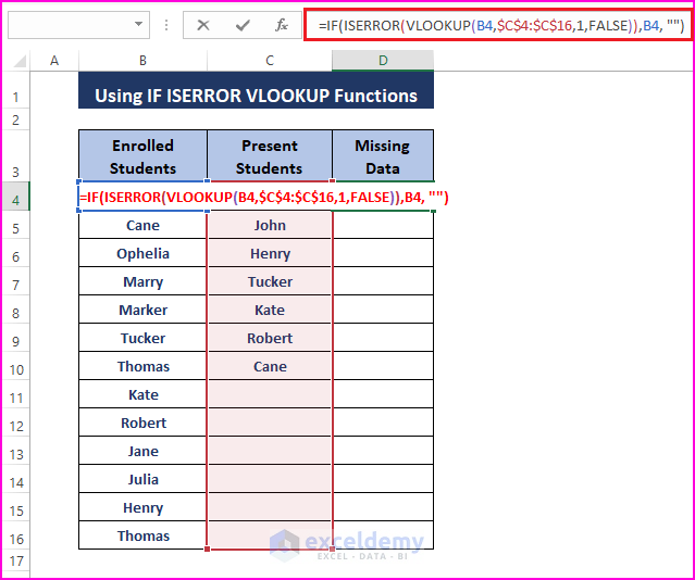
Formula Explanation
- The ISERROR(VLOOKUP(B4,$C$4:$C$16,1,FALSE) portion works as described in Method 1. Here, this portion is used as logical_test to display missing Cell Value (i,e., B4) or Blank Cell (i.e., “”) depending on the test outcomes; True or False respectively.
- Hit Enter to apply the formula.
- Drag the Fill Handle to display other missing entries.
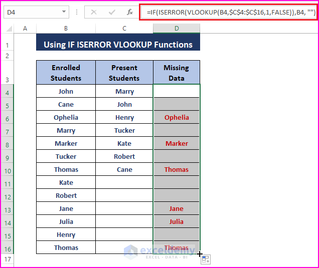
⧭Tips: Select the entire column, move to the Home tab, hover to the Font section, and choose any desired Font colors to highlight the fetched data.
Read More: How to Filter Missing Data in Excel
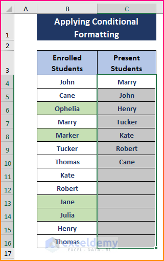
Method 4 – Conditional Formatting Unique Values to Highlight Missing Data
Steps:
- Highlight the columns containing different lists.
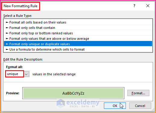
- Go to Conditional Formatting and choose New Rule.
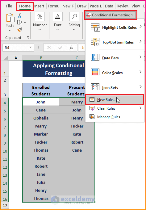
The New Formatting Rule window appears.
- Select Format only unique or duplicate values for Select a Rule Type.
- Choose Unique under Format all.
- Click Format and select a Fill Color.
- Click OK.
Excel highlights the unique values by comparing the adjacent column values as shown in the below image.
Read More: How to Compare Two Excel Sheets to Find Missing Data
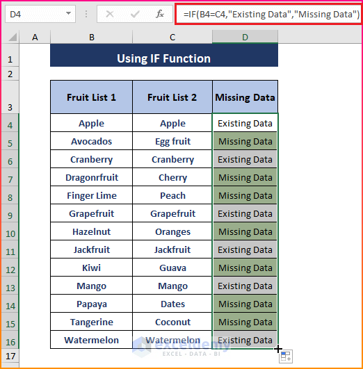
Method 5 – Using the IF Function to Cross Reference and Find Missing Data in Excel
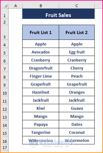
The following image depicts the fruit sales lists.
Steps:
- Insert the following formula to compare identical values among lists.
=IF(B4=C4,"Existing Data","Missing Data")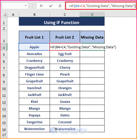
Formula Explanation
- The IF formula compares each B column entry to a C column entry to insert custom text such as “Existing Data” or “Missing Data”. B4=C4 acts as a logical_test and the formula inserts “Existing Data” if the test returns True otherwise “Missing Data”.
- Apply the formula using the Enter key, then use the Fill Handle to display the custom texts.
- Apply Conditional Formatting to the outcomes as depicted in the following image.
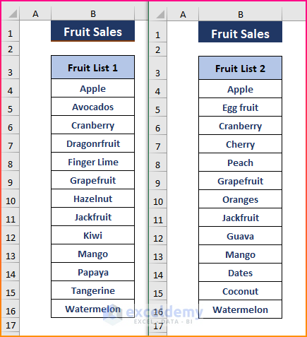
Method 6 – Cross Referencing Data from Different Worksheets to Find Missing Data+
The Fruit Lists may exist in different worksheets, as shown below.
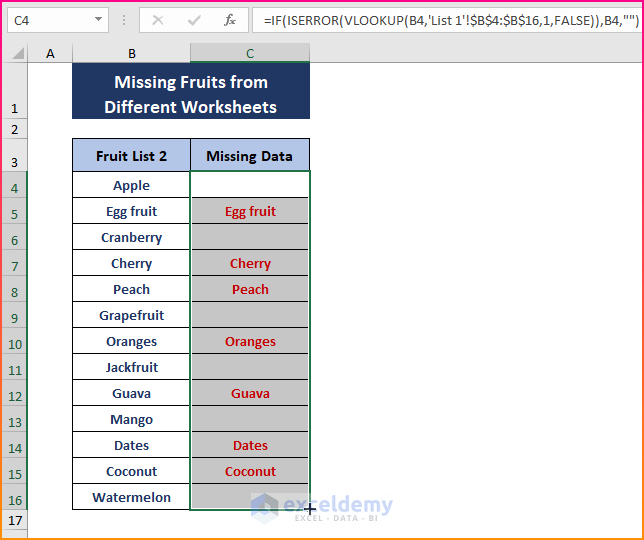
Steps:
- Add a helper column named Missing Data.
- Insert the following formula in any cells of the column.
=IF(ISERROR(VLOOKUP(B4,'List 1'!$B$4:$B$16,1,FALSE)),B4,"")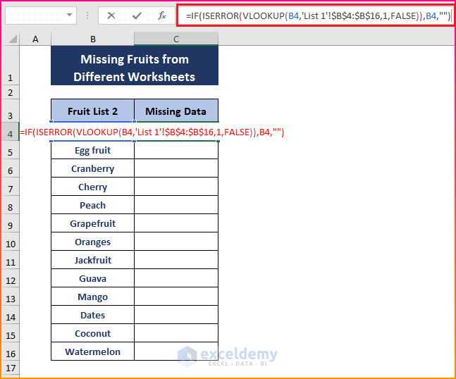
- Click Enter, then drag the Fill Handle to display the missing fruit names as shown in the below image.
- Reformat the cell if you want to display entries in custom formats.
Read More: How to Count Missing Values in Excel
Download the Excel Workbook
Related Articles
- How to Find Missing Rows in Excel
- How to Fill Missing Values in Excel
- How to Remove Missing Values in Excel
<< Go Back To Missing Values in Excel | Data Cleaning in Excel | Learn Excel
Get FREE Advanced Excel Exercises with Solutions!
