Sometimes, users have to list missing things in Microsoft Excel. While making these kinds of lists, it is important to count how many values are missing from the original data set. This is also helpful in moderating the attendance and activities of an institution’s employees. In this article, we will show you how to count missing values in Excel.
How to Count Missing Values in Excel: 2 Easy Ways
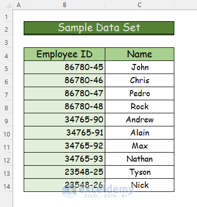
In this article, you will see two different and easy ways to count Missing Values in Excel. In our first approach, we will merge the COUNTIF function with the SUMPRODUCT function to count missing values. We will combine multiple functions for counting the missing values in Excel in our second method. For our working purposes, we will use the following data set.
1. Merging COUNTIF and SUMPRODUCT Functions to Count Missing Values
In our first method, we will merge the COUNTIF function with the SUMPRODUCT function to count missing values. Here we will count the number of missing employees in the same department of an institution on a working day. The COUNTIF function will determine the missing values one by one. Then, the SUMPRODUCT function will show the total missing values by adding them. For the detailed scenario, go through the following steps.
Step 1:
- First of all, make a list of the present employees for a particular day in column E.
- Here, we want to count how many employees from column C are missing from column E.
- Then, make the space where you want to count the missing values.
- In our example, it is cell C16.

Step 2:
- Secondly, type the following merged formula in cell C16.
=SUMPRODUCT(--(COUNTIF(E5:E12,C5:C14)=0))
Formula Breakdown
- COUNTIF(E5:E12,C5:C14): In this section, the COUNTIF function will look into cell range E5:E12. Then it will search for the same values in cell range C5:C14. If it finds any exact match then it will return the result as 1 otherwise 0. This function after looking through all the cells will give the result as {1,1,0,1,1,0,1,1,1,1}.
- (–(COUNTIF(E5:E12,C5:C14)=0)): The negative values will alter the result into {0,0,1,0,0,1,0,0,0,0}.
- SUMPRODUCT(–(COUNTIF(E5:E12,C5:C14)=0)): Finally, the SUMPRODUCT function will return the sum of the result of the previous steps which will be 2.
Step 3:
- Finally, after pressing Enter you will see the total missing employees from the list of column C which is 2.

Read More: How to Find Missing Values in a List in Excel
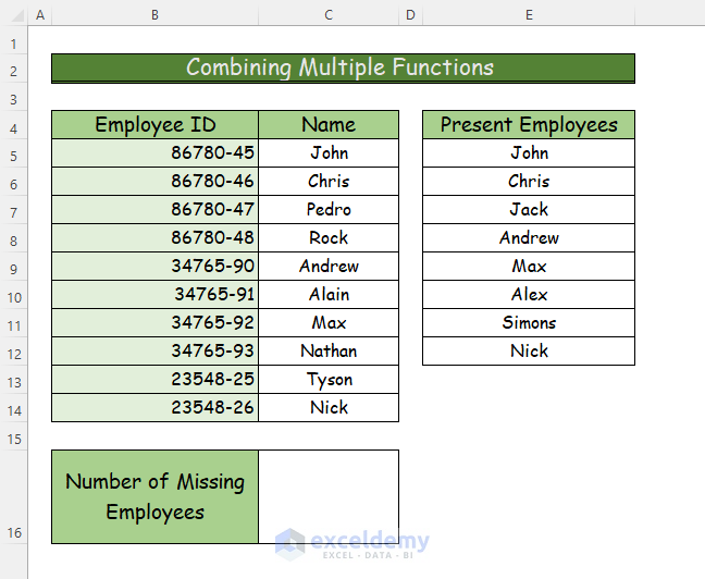
2. Combining Multiple Functions to Count Missing Values in Excel
In our second approach, the counting of missing values will be slightly different. Here, we will replace some employees and add some from other departments who are not present in the main data set. Then we will combine multiple functions to count how many employees from the main data set are missing. In the combination, we will use the MATCH function, the ISNA function, and the SUMPRODUCT function. The steps for this procedure are as follows.
Step 1:
- Firstly, edit the table in column E to add some employee names that are not included in the list in column C.
- Then, in cell C16, make the space to show the final result of this procedure.
Step 2:
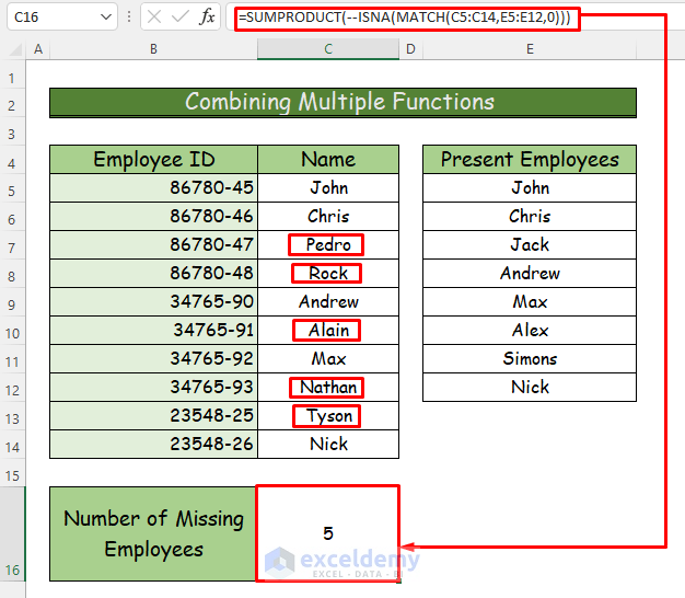
- Secondly, type the following formula, which is the combination of multiple functions.
=SUMPRODUCT(--ISNA(MATCH(C5:C14,E5:E12,0)))
Formula Breakdown
- MATCH(C5:C14,E5:E12,0): The MATCH function will look up the value from cell range C5:C14 then it will match those values in cell range E5:E12. Also, the match will be an exact match. That means if a value is not matched, it will result in #N/A. This will ultimately result in {1,2,#N/A,#N/A,4,#N/A,5,#N/A,#N/A,8}
- ISNA(MATCH(C5:C14,E5:E12,0)): The ISNA function will show True if it finds any error, otherwise it will show False. So the result will be {False,False,True,Ture,False,True,False,True,True, False}.
- SUMPRODUCT(–(COUNTIF(E5:E12,C5:C14)=0)): The negative signs will turn all the false values to 0 and all the trues to 1. Then the SUMPRODUCT function will return the missing value after adding all the 1s.
Step 3:
- Finally, press Enter and count all the missing values from column C.
- In our example, five values are missing from column C in contrast to column E.
Read More: How to Deal with Missing Data in Excel
Download Practice Workbook
You can download the free Excel workbook here and practice on your own.
Conclusion
That’s the end of this article. We hope you find this article helpful. After reading the above description, you will be able to count missing values in Excel by using any of the above-mentioned methods. Please share any further queries or recommendations with us in the comments section below.
Related Articles
- How to Fill Missing Values in Excel
- Compare Two Excel Sheets to Find Missing Data
- How to Cross Reference in Excel to Find Missing Data
- How to Remove Missing Values in Excel
- How to Filter Missing Data in Excel
- How to Find Missing Values in Excel
- How to Find Missing Rows in Excel
<< Go Back To Missing Values in Excel | Data Cleaning in Excel | Learn Excel
Get FREE Advanced Excel Exercises with Solutions!
