How to Filter Missing Data in Excel (4 Easy Methods)

This article will provide you with 4 easy methods to filter missing data in Excel.

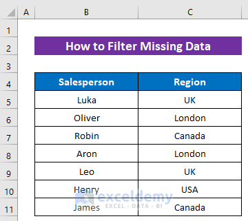
We’ll use the dataset below representing some salesperson’s sales regions to illustrate our methods.

Method 1 – Using the IF and COUNTIF Functions to Filter Missing Data

In our first method, we’ll apply the IF and COUNTIF functions to filter missing values from a list. If the value is found then our formula will return “Found”, and if not then it will return “Missing”.

Steps:

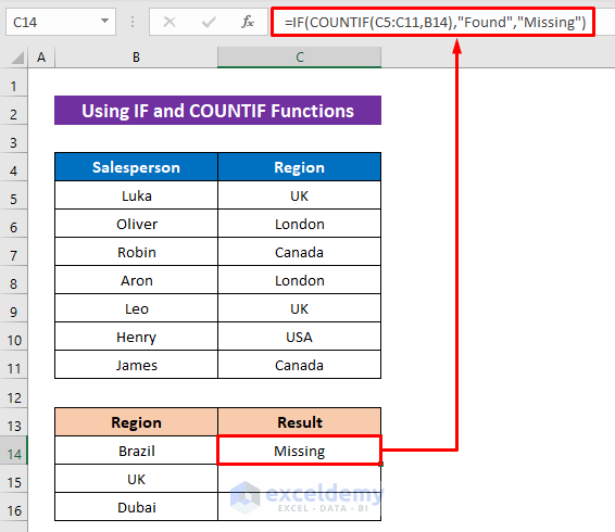
In cell C14 insert the following formula:

=IF(COUNTIF(C5:C11,B14),"Found","Missing")

Press ENTER to return the result.

Formula Breakdown:

COUNTIF(C5:C11,B14)

Counts the number of matching values in the range C5:C11.

IF(COUNTIF(C5:C11,B14),”Found”,”Missing”)

Returns “Missing” for 0 and “Found” for any greater number.

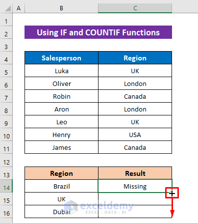
Drag down the Fill Handle icon to copy the formula to the cells below.

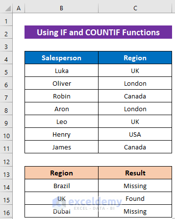
We were filtering for three values. We found one value, and two are missing.

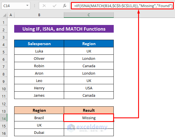
Method 2 – Using the IF, ISNA, and MATCH Functions to Filter Missing Data in Excel

The same operation can be performed using the IF, ISNA, and MATCH functions. We could use the ISERROR function instead of the ISNA function here to achieve the same result.

Steps:

Insert the following formula in cell C14:

=IF(ISNA(MATCH(B14,$C$5:$C$11,0)),"Missing","Found")

Press ENTER to return the result.

Formula Breakdown:

MATCH(B14,$C$5:$C$11,0)

Returns the row number from the list if the value matches, and the #N/A error if it doesn’t.

ISNA(MATCH(B14,$C$5:$C$11,0))

Returns TRUE for the #N/A error and FALSE for any other output.

IF(ISNA(MATCH(B14,$C$5:$C$11,0)),”Missing”,”Found”)

Returns Missing for TRUE and Found for False.

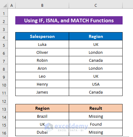
Use the Fill Handle tool to copy the formula to the cells below.

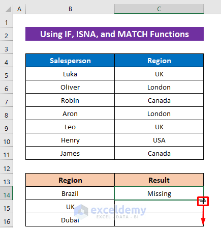
The same output as before is returned.

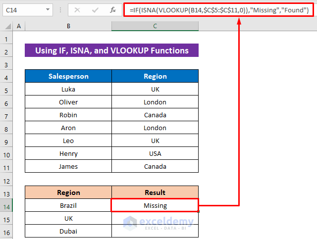
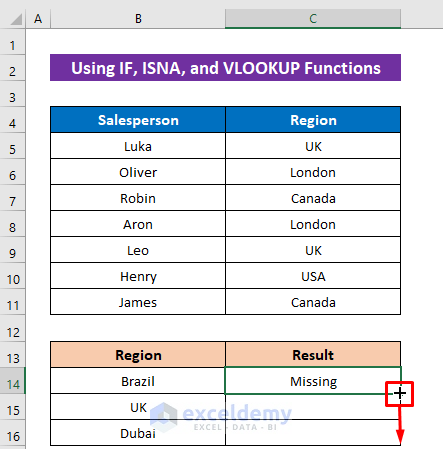
Method 3 – Using IF, ISNA, and VLOOKUP Functions

We’ll get the same result if we use the VLOOKUP function instead of the MATCH function in the previous formula.

Steps:

In cell C14, apply the following formula:

=IF(ISNA(VLOOKUP(B14,$C$5:$C$11,0)),"Missing","Found")

Press ENTER.

Formula Breakdown:

VLOOKUP(B14,$C$5:$C$11,1)

Here, the VLOOKUP function returns the lookup value if it matches and the #N/A error if doesn’t. Then the rest of the formula works like the previous formula.

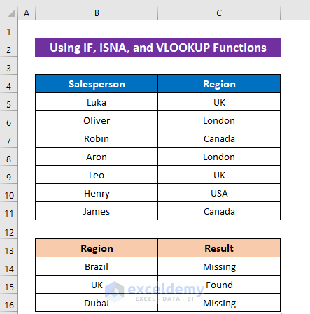
Apply the Fill Handle tool to copy the formula for the other regions.

The output will look like the image below.

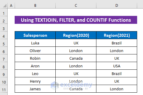
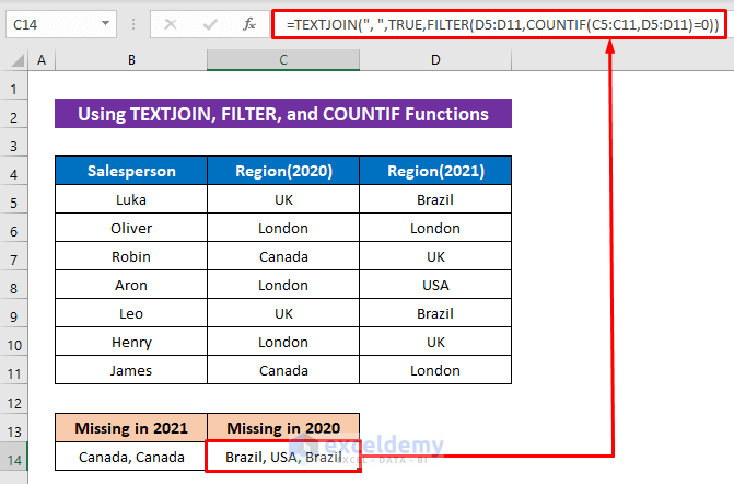
Method 4 – Using the TEXTJOIN, FILTER, and COUNTIF Functions to Filter Missing Data by Comparing Two Lists

In the previous methods, we filtered values from only one list. Now we’ll filter data from two lists (filtering one list’s data in another list) using the TEXTJOIN, FILTER, and COUNTIF functions. This formula will directly return the missing region names.

For this method, we modified the dataset to show the selling regions for two years in two columns.

Steps:

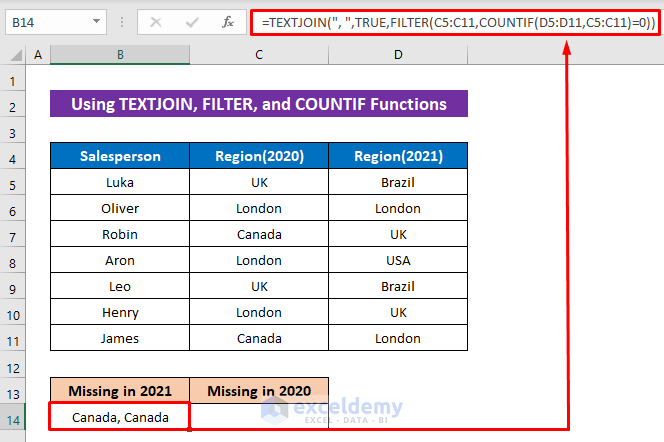
To filter for the regions of 2020 in 2021, enter the following formula in cell B14:

=TEXTJOIN(", ",TRUE,FILTER(C5:C11,COUNTIF(D5:D11,C5:C11)=0))

Press ENTER to return the region names.

Canada is returned twice because Canada was missing twice in 2020, and this formula doesn’t merge the same values.

Formula Breakdown:

COUNTIF(D5:D11,C5:C11)=0

Counts the number for each value in the range C5:C11 through the range D5:D11 and returns an array. If any value is equal to zero then it will return TRUE, and if not FALSE.