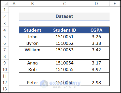
How to Remove Missing Values in Excel (7 Easy Methods)

Consider a dataset of student CGPAs with Student IDs. Some values are missing in Row 8 and Row 11. We’ll remove rows with missing data from the dataset.

Dataset

Method 1 – Applying the Go To Special Command

Steps:

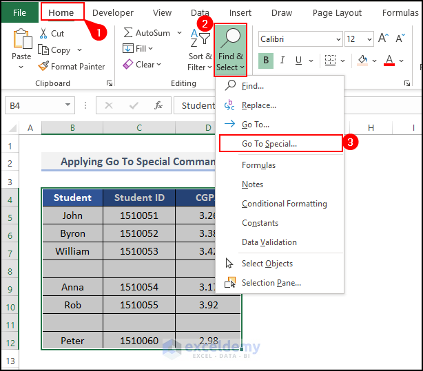
Select the entire range of your dataset.
Select Find & Select under the Home tab and click on Go To Special.

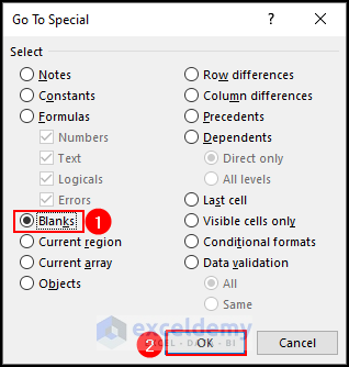
Applying Go To Special Command to Remove the missing values in Excel

A dialog prompt will appear named Go To Special. Select Blanks and hit OK.

Go To Special dialog box

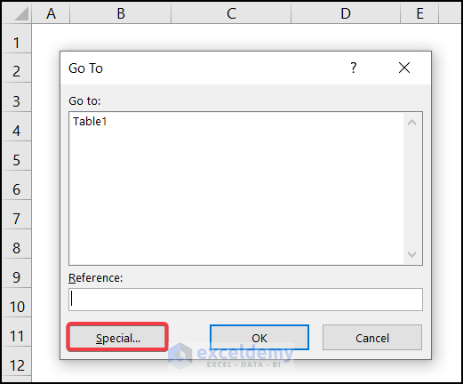
Alternatively, you can press Ctrl + G to get the Go To window, then choose the Special option or press Alt + S. You’ll get the Go To Special window as found earlier.

Inserting Go To Special

All the blank cells will be highlighted.
Right-click on any of the highlighted cells.
Select Delete from the Context Menu.

Deleting the blank rows

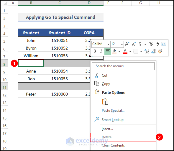
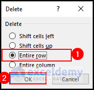
Pick Entire row from the Delete window.
Press OK.

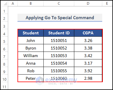
The blank rows will be removed.

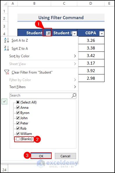
Method 2 – Using the Filter Command

Steps:

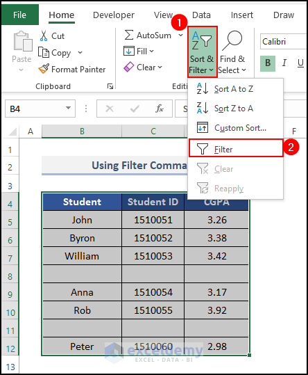
Select the entire range of your data and go to Sort & Filter, then select Filter.

Using Filter Command to remove missing values in Excel

Click on the Drop-down icon from any column and select (Blanks).
Press OK.

Drop down filter

The filter will hide rows that have empty cells in the selected column.

Filtered missing values

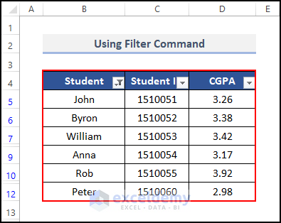
Note that the filter will also hide partially empty columns if you happen to filter by a column with a missing value.

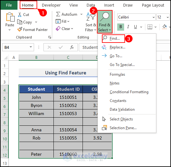
Method 3 – Utilizing the Find Feature

Steps:

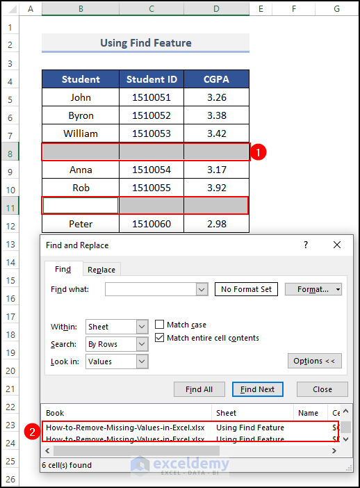
Select the whole data range and go to Find & Select.
Select Find.

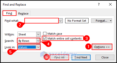
How to remove missing values in Excel by utilizing Find Feature

A dialog box will pop out (Find and Replace).
Go to Find and leave the Find what box empty.
Check the box before Match entire cell contents.
Select By Rows under the Search box, and select Values in the Look in box.
Select Find All.

Find and Replace

The dialog box will show you all the missing rows.
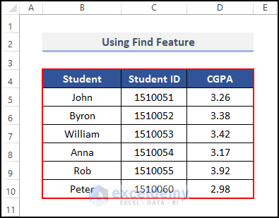
Select all the cells by pressing Ctrl + A, then delete them.

Utilizing Find Feature

This removes the missing data.

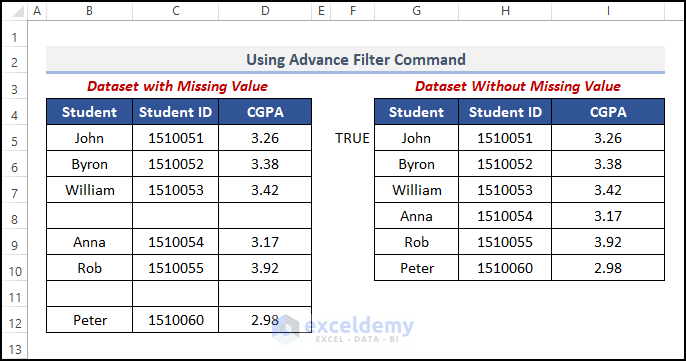
Method 4 – Applying an Advanced Filter

Steps:

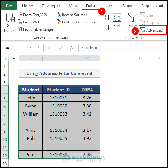
Select the whole dataset.
Go to the Data tab and select Advanced in the Sort & Filter group.

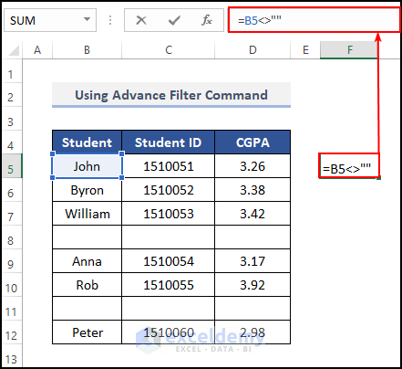
Applying Advanced Filter to remove missing values in Excel

Enter a value before going to the next steps. We entered B5<>” ”. The syntax will return TRUE if you have a value in the entire row you have selected.

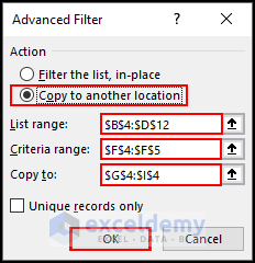
A dialog box will appear named Advanced Filter.
Select Copy to another location.
Put the List range as the dataset range: $B$4:$D$12.
Put the Criteria range as $F$4:$F$5 and Copy to as $G$4:$I$4.
Press OK.

Advance Filter dialog box

We’ll get a new table with filtered data.

how to remove missing values in Excel by using Advanced Filter

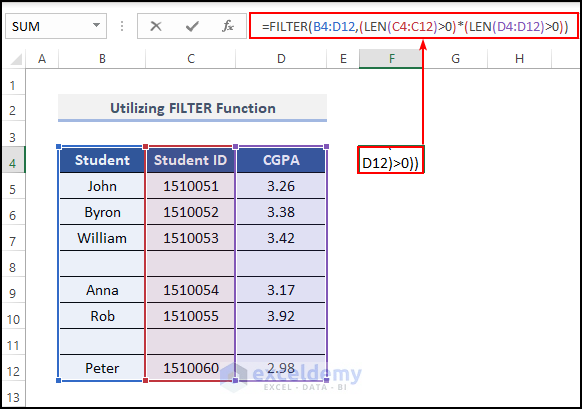
Method 5 – Utilizing the FILTER Function

Steps:

Select a blank cell where you want to enter the filtered table.
Insert the formula.

=FILTER(B4:D12,(LEN(C4:C12)>0)*(LEN(D4:D12)>0))

Formula Breakdown:

LEN function→ Counts the length of a string. Together with the greater than check, if the character length value is greater than 0, it will return TRUE. Otherwise, it will return FALSE. For values in empty rows, it will return FALSE.

FILTER function→ This function will filter the output of the LEN function and sort it. When the character length of a cell is 0, the cell is empty and the FILTER function will skip it.

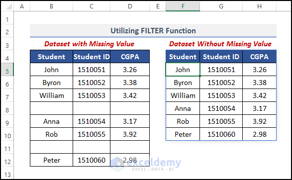
Press Enter.

Utilizing FILTER Function to remove missing values

Excel will create another data table without the missing values.

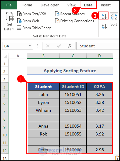
Method 6 – Applying the Sorting Feature

Steps:

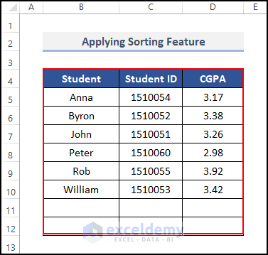
Select all the cells and go to the Data tab, then select the A→Z sort.

Applying sorting feature to remove missing values in Excel

This will send all the blank rows at the bottom of the data table. You can then hide them or discount them for future operations.

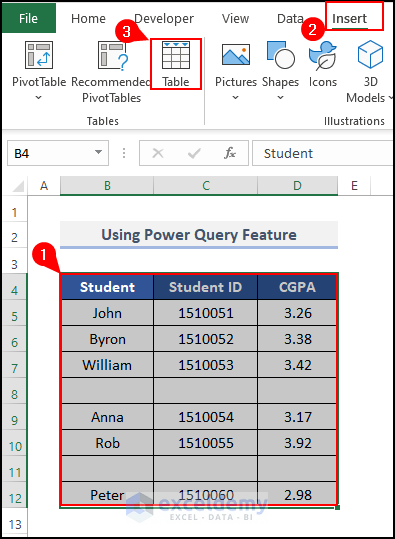
Method 7 – Using Power Query

Steps:

Select all the cells.
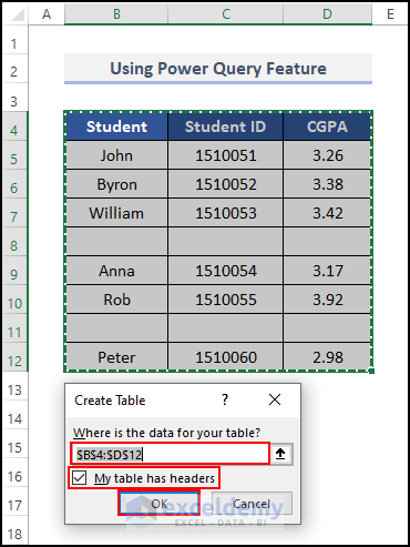
Go to the Insert tab and select Table.

how to remove missing values in Excel by employing Power Query Feature

Check My table has headers.
Press OK.

Creating a table

Go to the Data tab and select From Table/Range.

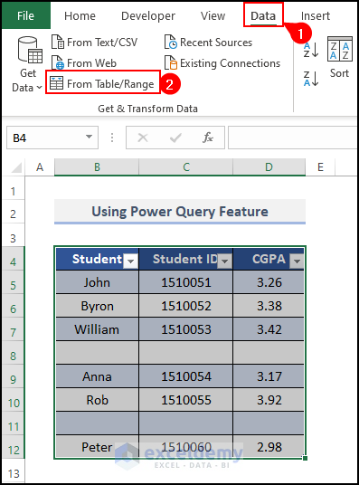
You’ll get a new window named Power Query Editor.
Select Reduce Rows, go to Remove Rows, and click on Remove Blank Rows.

Power Query editor

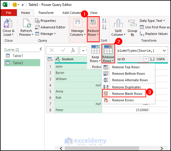
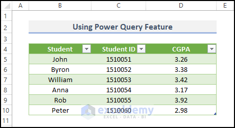
The editor will remove empty rows from the table.

Read More: How to Find Missing Rows in Excel

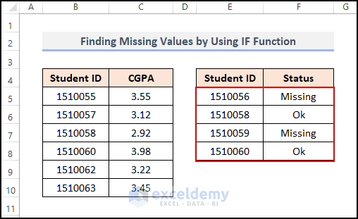
How to Find Missing Values in Excel

Steps:

We created a lookup table on the right of the original dataset, and listed the student IDs we want to check in column E.
Select cell F5 and insert the following formula:

=IF(COUNTIF(B5:C10,E5),”Ok”,”Missing”)

Formula Breakdown:

COUNTIF function→ checks whether data in E5 exists in the range B5:C10 and returns the number of appearances (or 0 for no match).

IF function→ if the value exists in the dataset, it gives the output OK. Otherwise, it will return Missing.

Press Enter.
AutoFill to the rest of the column.

How to Find Missing Values in Excel

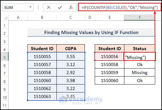
Here’s the result.

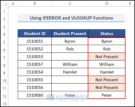
How to Deal with Missing Data in Excel

Steps:

Select cell D5 and insert the following formula:

=IFERROR(VLOOKUP(C5,$C$5:$C$12,1,0),”Not Present”)

Formula Breakdown:

The VLOOKUP function considers C5 as the lookup_value and $C$5:$C$12 as the lookup array, 1 as col_index_num, and 0 as range lookup.

The IFERROR function returns Not Present if it finds an error or the value of column C if it doesn’t find an error. So, when the LOOKUP function doesn’t find a value and makes an error, the IFERROR function returns Not Present, otherwise, it will return the same value as column C.

Press Enter.
AutoFill the formula to the rest of the column.

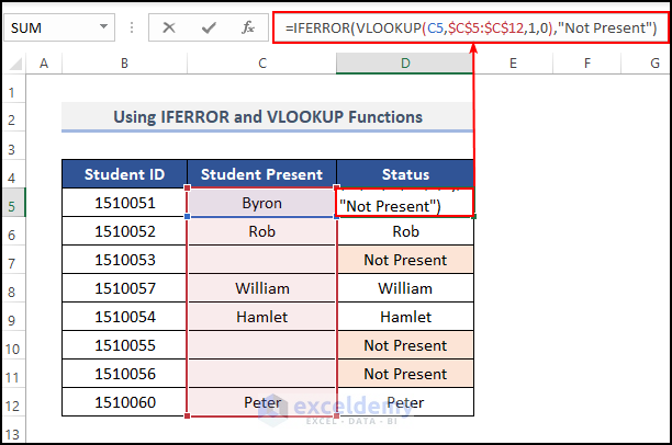
How to Deal with Missing Data in Excel

We declare the missing value as “Not Present”. You can also highlight them.

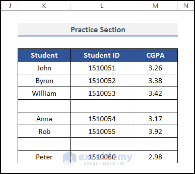
Practice Section

We have provided a practice section on each sheet on the right side so you can test out these methods on the sample set or make changes and see how the formulas function.

Practice Section