ANOVA provides a perfect opportunity to evaluate which factor has the most significant effect on a given set of data. It stands for analysis of variance just like a t-test. There are many ways through which you can do ANOVA analysis in Excel. This article will show how to do one way ANOVA in Excel. I hope you find this article interesting and gain complete knowledge regarding one-way ANOVA.
What Is ANOVA Analysis?
ANOVA is known as the analysis of variance. It is a statistical method that is used to analyze variance within the dataset. After completing the analysis, an analyst usually performs extra analysis on the methodological factors that impact significantly the inconsistent nature of the data sets. In that case, you can use ANOVA which compares many data sets simultaneously to see whether there is a link between them.
What Is One Way ANOVA?
There are two types of ANOVA: single factor and two factors. The one-way ANOVA determines whether there is a significant difference between the mean of three or more groups. It also compares the mean between groups The basic difference between one-way ANOVA and two-way ANOVA is the number of independent variables. The independent variables divide the individual groups into two or more levels. The one-way ANOVA can’t tell you which specific groups are statistically different from each other but it tells which two groups are different.
How to Do One Way ANOVA in Excel: 2 Suitable Examples
To do one-way ANOVA in Excel, we have taken two different examples through which you can have a complete solution. Here, we take some students’ marks and sales amounts to do a one-way ANOVA in Excel. Before doing anything, you need to enable the Data Analysis tool. After that, you can apply the one-way ANOVA in Excel.
1. How to Do One Way ANOVA in Excel for Student Marks
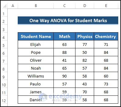
For the first example, we take a dataset that includes some students and their marks in math, physics, and chemistry.
Step 1: Enable Data Analysis ToolPak
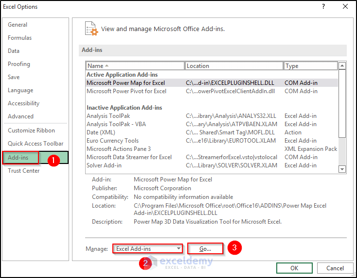
First, you need to enable Data Analysis Toolpak using Excel options. Without enabling this, you can’t use the data analysis option to do one-way ANOVA in Excel.
- Go to the File tab in the ribbon.
- Then, go to the More command.
- From there, select Options.

- It will open the Excel Options dialog box.
- Then, select the Add-ins option.
- After that, select Excel Add-ins from the Manage section.
- Then, select Go.
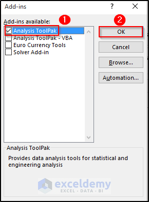
- As a result, the Add-ins dialog box will appear.
- Then, select Analysis ToolPak from the Add-ins Available section.
- Finally, click on OK.
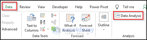
- As a result, you will see the Data Analysis option under the Analysis group.

Step 2: Do One Way ANOVA in Excel
In this step, we will do the one-way ANOVA in Excel. In this step, we will use the Data Analysis tool to do the one-way ANOVA in Excel.
- First, go to the Data tab in the ribbon.
- Then, select Data Analysis from the Analysis group.
- It will open the Data Analysis dialog box.
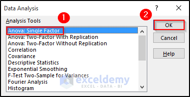
- Then, select Anova: Single Factor from the Analysis Tools section.
- Finally, click on OK.
- As a result, the Anova: Single Factor dialog box.
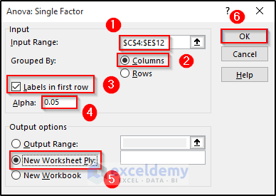
- Then, set the input range.
- Check on the Columns from the Grouped By section.
- Then, check on the Labels in first row.
- After that, set Alpha as 05.
- We want to show our output in a new worksheet. So, select New Worksheet Ply.
- Finally, click on OK.
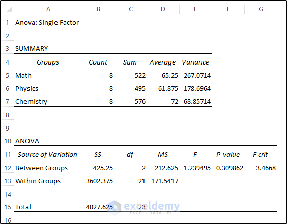
- After clicking the OK, the Anova: Single Factor will show its result in a new worksheet. See the screenshot.
Interpretation of the Result
In the summary table, we will find four results: Count, Sum, Average, and Variance. The Count section denotes the number of data of each group. The Sum section denotes the total value of the given data while adding them. The Average denotes the mean value of each group. In the summary, you can see the groups have the highest average for Chemistry and the highest variance obtained from Math.
ANOVA analysis determines the null hypothesis in the data. In the ANOVA table, you will see the results of two types: Between Groups and Within Groups. In this table, ANOVA calculates Test Statistics (F), P value, and Critical Value (F crit). Before interpreting the result, we have to know the criteria.
- When the test statistic is greater than the critical value (e F>F crit), then, it rejects the null hypothesis which means the means are different.
- When the test statistics are lower than the critical value (e F<F crit), then it accepts the null hypothesis which means the means are not different.
- In terms of the P value, if the P value is less than Alpha, it rejects the null hypothesis.
- If the P value is greater than Alpha, it accepts the null hypothesis.
In this example, the test statistic (1.2394) is lower than the critical value (3.4668), so, it accepts the null hypothesis. In terms of the P value, the P value is greater than the Alpha, so, it also accepts the null hypothesis. That means there is no difference between the mean of the three groups.
2. How to Do One Way ANOVA in Excel for Sales Amount
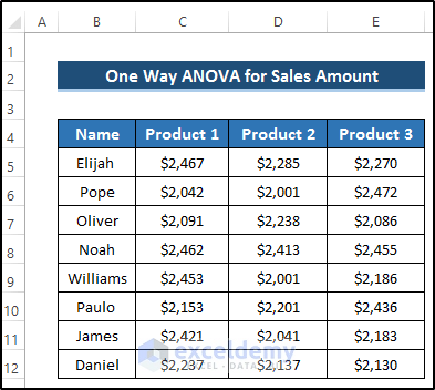
For the second example, we take a dataset that includes some salesperson and their sales amount for three different products. Now, we want to show how to do one way ANOVA in Excel and analyze these three products’ sales amounts and finally find out the required output.
Step 1: Enable Data Analysis Toolpak
First, you need to enable Data Analysis Toolpak using Excel options. Without enabling this, you can’t use the data analysis option to do one-way ANOVA in Excel.
- Go to the File tab in the ribbon.
- Then, go to the More command.
- From there, select Options.
- It will open the Excel Options dialog box.
- Then, select the Add-ins option.
- After that, select Excel Add-ins from the Manage section.
- Then, select Go.
- As a result, the Add-ins dialog box will appear.
- Then, select Analysis ToolPak from the Add-ins Available section.
- Finally, click on OK.
- As a result, you will see the Data Analysis option under the Analysis group.
Step 2: Do One Way ANOVA in Excel
In this step, we will do the one-way ANOVA in Excel. In this step, we will use the Data Analysis tool to do the one-way ANOVA in Excel.
- First, go to the Data tab in the ribbon.
- Then, select Data Analysis from the Analysis group.
- It will open the Data Analysis dialog box.
- Then, select Anova: Single Factor from the Analysis Tools section.
- Finally, click on OK.
- As a result, the Anova: Single Factor dialog box.
- Then, set the input range.
- Check on the Columns from the Grouped By section.
- Then, check on the Labels in first row.
- After that, set Alpha as 05.
- We want to show our output in a new worksheet. So, select New Worksheet Ply.
- Finally, click on OK.
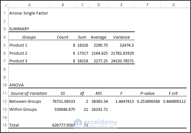
- After clicking the OK, the Anova: Single Factor will show its result in a new worksheet. See the screenshot.
Interpretation of the Result
In the summary table, we will find four results: Count, Sum, Average, and Variance. The Count section denotes the number of data of each group. The Sum section denotes the total value of the given data while adding them. The Average denotes the mean value of each group. For the summary, you can see the groups have the highest average from product 3 and the highest variance obtained from Product 1.
ANOVA analysis determines the null hypothesis in the data. In the ANOVA table, you will see the results of two types: Between Groups and Within Groups. In this table, ANOVA calculates Test Statistics (F), P value, and Critical Value (F crit). Before interpreting the result, we have to know the criteria.
- When the test statistic is greater than the critical value (e F>F crit), then, it rejects the null hypothesis which means the means are different.
- When the test statistics are lower than the critical value (e F<F crit), then it accepts the null hypothesis which means the means are not different.
- In terms of the P value, if the P value is less than Alpha, it rejects the null hypothesis.
- If the P value is greater than Alpha, it accepts the null hypothesis.
In this example, the test statistic (1.46) is lower than the critical value (3.4668), so, it accepts the null hypothesis. In terms of the P value, the P value (0.2538) is greater than Alpha (0.05), so, it also accepts the null hypothesis. That means there is no difference between the mean of the three groups.
Download Practice Workbook
Download the practice workbook below.
Conclusion
We have shown two different examples through which you can have a clear view of how to do one way ANOVA in Excel. Both of these examples are fairly easy to understand and at the same time, it provides the required valuable outputs. I think we covered all the possible areas regarding the one-way ANOVA in Excel. If you have further questions, feel free to ask in the comment box.
Related Articles
- How to Interpret ANOVA Single Factor Results in Excel
- How to Do Repeated Measures ANOVA in Excel
- How to Apply Rows Per Sample ANOVA in Excel
- Randomized Block Design ANOVA in Excel
- Two Way ANOVA in Excel with Unequal Sample Size
- How to Use Two Factor ANOVA with Replication in Excel
- How to Use ANOVA Two Factor Without Replication in Excel
- How to Interpret Two-Way ANOVA Results in Excel
<< Go Back to Anova in Excel | Excel for Statistics | Learn Excel
Get FREE Advanced Excel Exercises with Solutions!
