In the modern era of data analysis, you may be required to calculate the P value in Excel. You can do this using one way ANOVA or two way ANOVA. In this article, we are going to demonstrate to you 3 possible ways to calculate the P value in Excel ANOVA. If you are curious about it, download our practice workbook and follow us.
What Is ANOVA Analysis?
ANOVA provides us with the first opportunity to determine which factors have a significant effect on a dataset. After completing the analysis, an analyst does extra analysis on the methodological factors that significantly impact the inconsistent nature of that data set. Additionally, he uses the Anova analysis findings in the f-test to create extra data relevant to the estimated regression analysis. The ANOVA analysis compares many data sets simultaneously to see whether there are any connections among them. ANOVA is a statistical method used to analyze variance observed within a dataset by dividing it into two sections:
-
-
-
-
-
-
-
-
-
-
-
-
- Systematic factors and
- Random factors
-
-
-
-
-
-
-
-
-
-
-
The mathematical formula for Anova is:

Here,
- F = Anova Coefficient,
- MST = Mean Sum of Squares Due to Treatment,
- MSE = Mean Sum of Squares Due to Error.
What Is P Value?
The P value represents the probability value of any dataset. If the null hypothesis is true, the likelihood of receiving findings from a statistical hypothesis test that are at least as severe as the actual results is known as the P-value. The smallest level of significance at which the null hypothesis would be rejected is provided by the P-value as an alternative to rejection points. Stronger support for the alternative hypothesis is indicated by a lower P-value.
How to Calculate P Value in Excel ANOVA: 3 Suitable Examples
To demonstrate the examples, we consider a dataset of two samples. We take four students’ examination marks in math and chemistry from two shifts of any institution. So, we can claim that our dataset is in the range of cells B5:D12.

1. Using Single Factor ANOVA Analysis
In the first example, we will show you the procedure to calculate the P value using Anova: Single Factor. The steps of this method are given below:
📌 Steps:
- First of all, from the Data tab, select the Data Toolpak from the group Analysis. If you don’t have the Data Toolpak in the Data tab, you can enable it from the Excel Options.

- As a result, a small dialog box called Data Analysis will appear.
- Now, select the Anova: Single Factor option and click OK.

- Another dialog box called Anova: Single Factor will appear.
- Then, in the Input section, select the input cell range of the dataset. Here, the Input Range is $C$5:$D$12.
- Keep the Grouped by option in Columns.
- After that, in the Output section, you have to specify how you want to get the result. You can get it in three different ways. We want to get the result on the same sheet.
- So, we choose the Output Range option and denote the cell reference as $F$4.
- Finally, click OK.

- Within a second, you will get the result. Our desired P value is in cell K14. Besides that, you will also get a summary result in the range of cells F6:J9.
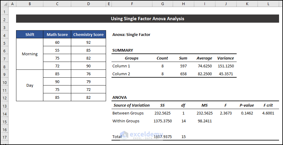
Thus, we can say that our method worked perfectly, and we were able to calculate the P value in Excel Anova.
🔎 Interpretation of the Result
In this example, we got a P value of 0.1462. It means that the possibility of getting a similar number in both groups is 0.1462 or 14.62%. So, we can claim that this P value has significance in our chosen dataset.
2. Utilizing Two-Factor with Replication ANOVA Analysis
In the following example, we are going to use the Anova: Two-Factor with Replication process to calculate the P value of our dataset. The steps of this approach are given as follows:
📌 Steps:
- First, in the Data tab, select the Data Toolpak from the group Analysis. If you don’t have the Data Toolpak in the Data tab, you can enable it from the Excel Options.

- As a result, the Data Analysis dialog box will appear.
- After that, choose Anova: Two-Factor With Replication and click OK.

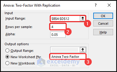
- Another small dialog box called Anova: Two-Factor With Replication will appear.
- Now, in the Input section, select the input cell range of the dataset. Here, the Input Range is $B$4:$D$12.
- Then, denote the Rows per sample field as 4.
- Afterward, in the Output section, you have to mention how you want to get the result. You can get it in three different ways. In this example, we want to get the result in a new worksheet.
- Thus, choose the New Worksheet Ply option and write down a suitable name according to your desire. We write Anova Two Factor to get a new worksheet of this name.
- Finally, click OK.
- You will notice a new worksheet will be created, and Excel will show the analysis result on that worksheet. Our desired P value is in the range of cells G25:G27. Besides that, you will also get a summary result in the range of cells B3:D20.
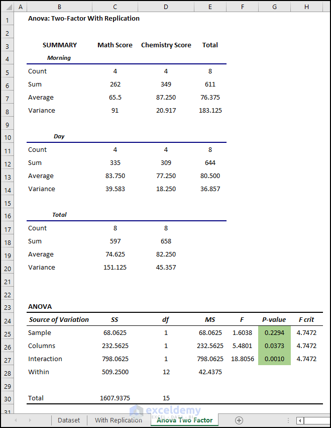
Hence, we can say that our method worked effectively, and we were able to calculate the P value in Excel Anova.
🔎 Interpretation of the Result
In this example, the P-value for the Columns is 0.0373, which is statistically significant, so we can say that there is an effect of shifts on the performance of the students in the exam. But the 3rd image of the example procedure shows that the value is close to the alpha value of 0.05, so the effect is less significant.
Similarly, the P-value of Interactions is 0.0010, which is much less than the alpha value, so it has statistically high significance, and we can remark that the effect of the shift on both exams is very high.
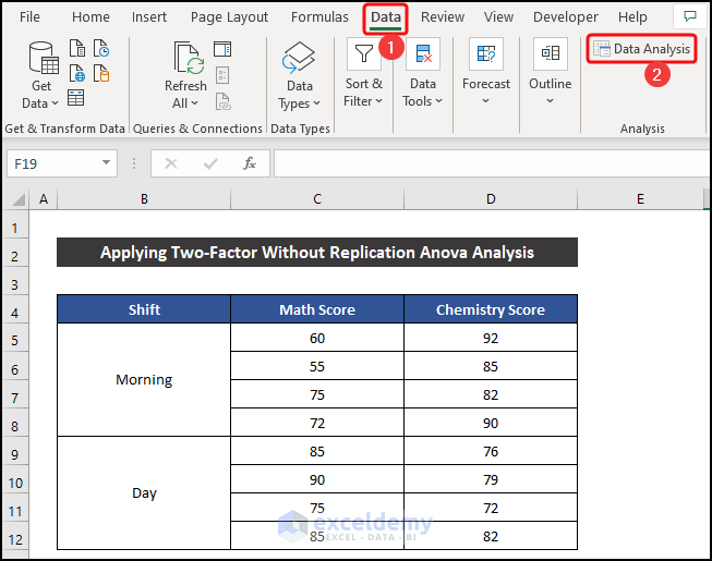
3. Applying Two-Factor Without Replication ANOVA Analysis
In this example, the Anova: Two-Factor Without Replication will help us calculate the P value. The procedure is described below step-by-step:
📌 Steps:
- Firstly, in the Data tab, select the Data Toolpak from the group Analysis. If you don’t have the Data Toolpak in the Data tab, you can enable it from the Excel Options.
- As a result, a small dialog box called Data Analysis will appear.
- Next, select the Anova: Two-Factor Without Replication option and press OK.

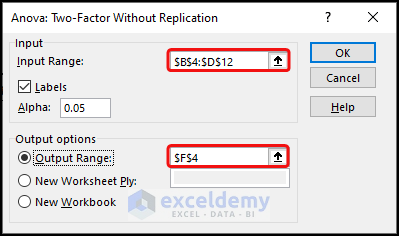
- Another small dialog box called Anova: Two-Factor Without Replication will appear.
- After that, in the Input section, choose the input cell range of the dataset. Here, the Input Range is $B$4:$D$12.
- Then, check the Labels option if it is not checked yet.
- Now, in the Output section, you have to specify how you want to get the result. You can get it in three different ways. We want to get the result in the same sheet.
- Hence, we choose the Output Range option and denote the cell reference as $F$4.
- Finally, click OK.
- Within a second, you will notice the result shown from cell F4. Our desired P value is in the range of cell K22:K23. Besides that, you will also get a summary result in the range of cells F6:J17.
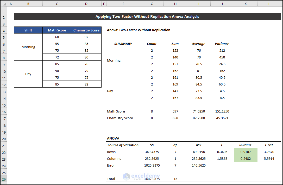
Finally, we can say that our method worked successfully, and we were able to calculate the P value in Excel Anova.
🔎 Interpretation of the Result
Here, the P-value for Columns is 0.2482, which is statistically significant. So, we can say that there is an effect of shifts on the performance of the students in the examination. However, the value is close to the alpha value of 0.05, so the effect is less significant.
Read More: How to Interpret Two-Way ANOVA Results in Excel
Download Practice Workbook
Download this practice workbook for practice while you are reading this article.
Conclusion
That’s the end of this article. I hope that this article will be helpful for you and you will be able to calculate the P value in Excel Anova. Please share any further queries or recommendations with us in the comments section below if you have any further questions or recommendations.
Keep learning new methods and keep growing!
Related Articles
- Nested ANOVA in Excel
- How to Interpret ANOVA Single Factor Results in Excel
- How to Interpret ANOVA Results in Excel
- How to Make an ANOVA Table in Excel
- How to Perform Regression in Excel and Interpretation of ANOVA
- How to Graph ANOVA Results in Excel
<< Go Back to Anova in Excel | Excel for Statistics | Learn Excel
Get FREE Advanced Excel Exercises with Solutions!
