Introduction to ANOVA in Excel
ANOVA is the abbreviation of Analysis of Variance. In Excel, it is a method to obtain the values required to test the Null Hypothesis. Excel allows us to apply this method for:
- ANOVA: Single Factor
- ANOVA: Two-Factor With Replication
- ANOVA: Two-Factor Without Replication
The single factor is applicable when there are multiple data samples and you need to perform the hypothesis test for differences in those samples only.
The two-factor with replication applies when each sample data is divided into similar groups, and you need to perform the hypothesis test for differences within those groups and within different samples.
The two-factor without replication applies when you need to perform the hypothesis test difference within each sample and within different samples.
You can create an Anova table using the Data Analysis tool in Excel. To activate the tool:
- Go to File>>Options or press ALT+F+T.
- Select the Add-ins tab>>Manage Excel Add-ins>>Go.
- Check Analysis ToolPak >>Click OK.
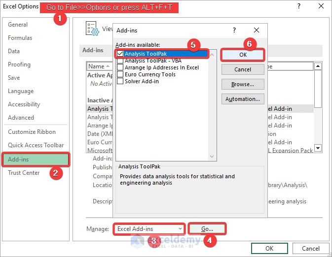
You will be able to access the Data Analysis tool from the Data tab.

Method 1 – Using the ‘ANOVA: Single Factor’ to Create an ANOVA Table in Excel
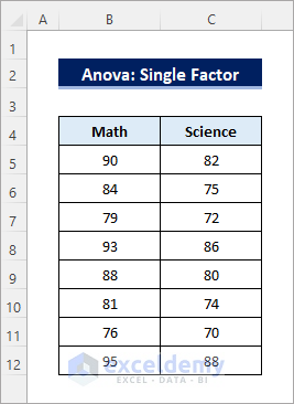
The dataset contains marks obtained by a group of students in two different tests.
To analyze the dataset and find if there are any significant differences between the test results:
Perform the one-way or single-factor ANOVA.
Steps:
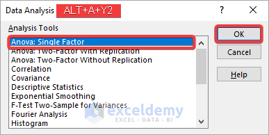
- Select Data>>Data Analysis.
- Choose Anova: Single Factor in the analysis toolbox and click OK.
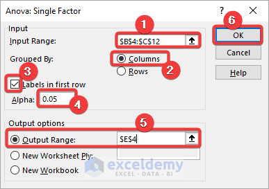
- In the Anova: Single Factor dialog box, select the entire dataset including the labels (B4:C12) in Input Range.
- Select Columns beside Grouped By.
- Check Labels in first row.
- Keep the Alpha value to 0.05.
- Select Output Range and enter the cell reference to create the Anova table.
- Click OK.
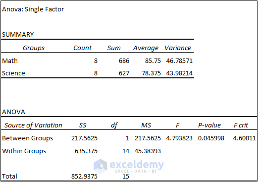
You will see the following table in the output location.
Method 2 – Utilizing the ‘Anova: Two-Factor With Replication’ Option
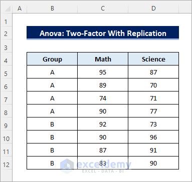
You have a similar dataset. The students are divided into two different groups.
To see if there is any significant difference in performance between the two groups:
Perform a two-way or two-factor ANOVA with replication.
Steps:
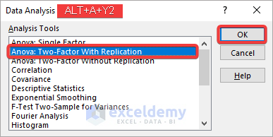
- Select Data>>Data Analysis.
- Choose Anova: Two-Factor With Replication in the analysis toolbox and click OK.
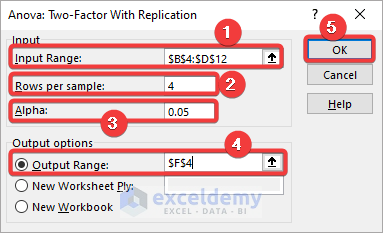
- In the Anova: Two-Factor With Replication dialog box, select the entire dataset including the labels (B4:D12) in Input Range.
- Enter 4 in Rows per sample.
- Keep the Alpha value to 05.
- Select Output Range and enter the cell reference to create the Anova table.
- Click OK.
You will see the following table in the output location.
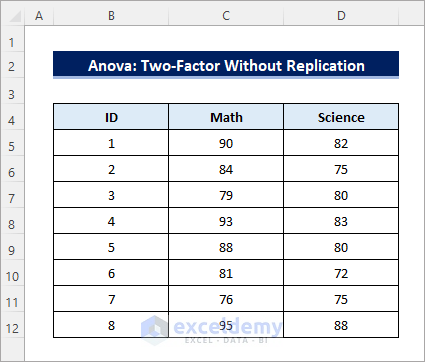
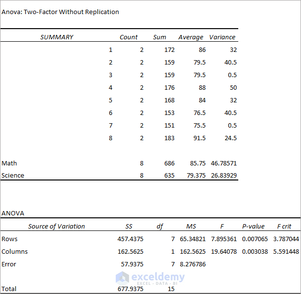
Method 3 – Using the ‘Anova: Two-Factor Without Replication’ Option to Create an ANOVA Table
Find if there are significant differences among individual performances along with the test-wise performances:
Steps:
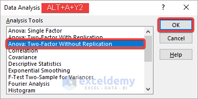
- Select Data>>Data Analysis.
- Choose Anova: Two-Factor Without Replication in the analysis toolbox and click OK.
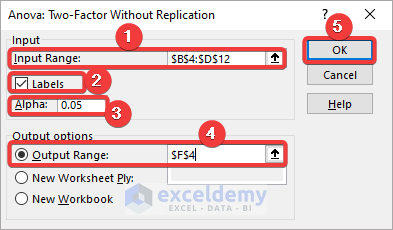
- In the Anova: Two-Factor Without Replication dialog box, select the entire dataset including the labels (B4:D12) in Input Range.
- Check Labels.
- Keep the Alpha value to 0.05.
- Select Output Range and enter the cell reference to create the Anova table.
- Click OK.
You will see the following table in the output location.
How to Interpret an ANOVA Table in Excel
We perform variance analysis to test if the Null Hypothesis is true for a dataset. The Null Hypothesis suggests that two sets of data are the same and the difference between them is insignificant. We can decide whether this hypothesis is true, considering three properties in the Anova table:
- F-value
- F crit-value
- P-value
Check if the F-value is higher or lower than the F critical value. F > F crit rejects the Null Hypothesis and indicates that the two possibilities are not the same.
P-value<Alpha (0.05) also rejects the Null Hypothesis indicating that the difference between the two sets of data is statistically significant.
1. Read the Single Factor Analysis Results
Observe the Anova table obtained from the Single Factor Anova test.
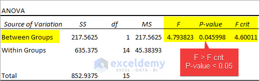
- F(4.793823)>F crit(4.60011) suggests that there is a difference between individual performances. P-value<0.05 suggest that the difference between individual performances is statistically significant.
Read More: How to Calculate P Value in Excel ANOVA
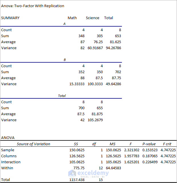
2. Read the Two-Factor With Replication Analysis Results
Observe the Anova table obtained from the Two-Factor with Replication ANOVA test.
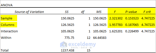
- F(2.321302)<F crit(4.747225) for Sample accepts the Null Hypothesis and indicates that group performances are the same. P-value>>0.05 also accepts the Null Hypothesis and indicates that the difference in group performances is statistically insignificant.
- F(1.957783)<F crit(4.747225) for Columns accepts the Null Hypothesis and indicates that group performances between the two tests (Math & Science) are the same. P-value<<0.05 suggests that the difference in group performances between the two tests is statistically insignificant.
Read More: How to Interpret Two-Way ANOVA Results in Excel
3. Interpret The Two-Factor Without Replication Analysis Output
Observe the Anova table obtained from the Two-Factor With Replication Anova test.
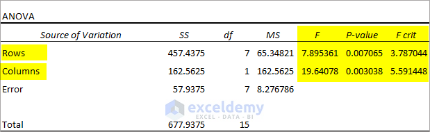
- F(7.895361)>F crit(3.787044) for Rows suggests that there is a difference between individual performances. P-value<<0.05 suggests that the difference between individual performances is statistically significant.
- F(19.64078)>>F crit(5.591448) for Columns suggests that there is a huge difference in performances between the two tests (Math & Science). P-value<<0.05 suggests that the difference in performance between the two tests is statistically significant.
Read More: How to Interpret ANOVA Results in Excel
Download Practice Workbook
Download the practice workbook.
Related Articles
- Nested ANOVA in Excel
- Two Way ANOVA in Excel with Unequal Sample Size
- How to Perform Regression in Excel and Interpretation of ANOVA
- How to Graph ANOVA Results in Excel
<< Go Back to Anova in Excel | Excel for Statistics | Learn Excel
Get FREE Advanced Excel Exercises with Solutions!
