How to Do ANOVA in Excel (2 Suitable Examples)

If you are looking for ways to do ANOVA in Excel, then this article will serve this purpose. ANOVA is used to find differences among groups of data that are statistically different. In Excel, we can do ANOVA by following some simple steps. So let’s start with the article and learn all these steps to do ANOVA in Excel.

What Is ANOVA?

ANOVA is the acronym for Analysis of Variance. It is a statistical test. In 1918, Ronald Fisher first developed this method. It is a statistical approach that separates variance into different components so that they can be used in further tests. There are several types of ANOVA. In this article, we will 2 types of ANOVA. They are:

One Way ANOVA
Two Way ANOVA

How to Do ANOVA in Excel: 2 Suitable Examples

In this section of the article, we are going to learn about the detailed steps of 2 methods to do ANOVA in Excel.
We have used Microsoft Excel 365 version for this article, you can use any other version according to your convenience.

1. One Way ANOVA in Excel

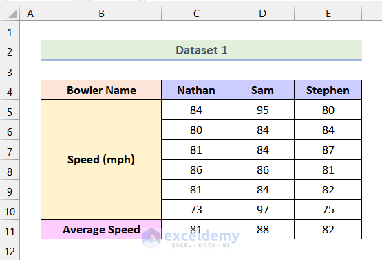
In the following dataset, we have the bowling Speed of 3 Bowlers and their Average Speed. Here, there is only one variable that influences bowling speed. That is, depending on the bowler, the speed varies. Our aim is to do a one way ANOVA test with this data.

Step 01: Adding Analysis ToolPak

To do ANOVA, we need to have a Data Analysis option. By default, the Data Analysis feature is not added in Excel. We need to manually add the Analysis ToolPak Add-in to enable this feature.

Firstly, press the keyboard shortcut ALT + F + T to open the Excel Options dialogue box from your worksheet.

Following that, go to the Add-ins tab.
After that, click on the Go option as marked in the following picture.

Now, from the Add-ins dialogue box, check the box of Analysis ToolPak.
Next, click OK.

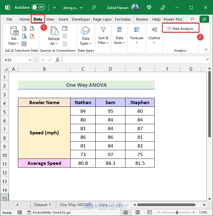
Now go to the Data tab from the Ribbon. You will see that there is a Data Analysis option at the top right side of the Ribbon.

Step 02: Doing ANOVA Test

After the Data Analysis option has been enabled, we will follow the steps mentioned below to do ANOVA.

Firstly, go to the Data tab from the Ribbon.
After that, click on the Data Analysis option.

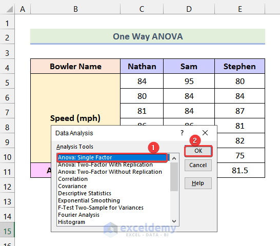
As a result, the Data Analysis dialogue box will open as shown in the image given below.

Now, from the Data Analysis dialogue box, choose Anova: Single Factor.
Subsequently, click OK.

Afterward, the Anova: Single Factor dialogue box will be available on your worksheet as demonstrated in the following image.

Now, click on the Input Range box.
Following that, select the dataset as marked in the following picture.
Then check the box of Labels in first row.

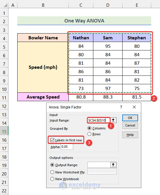
Next, click on the Output Range box.
After that, select the cell from where you want to display the output. In this case, we have selected cell B14.
Finally, click OK.

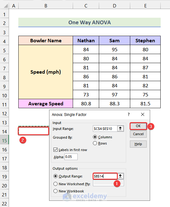
Consequently, you will see the outputs of the ANOVA test as demonstrated in the following picture.

2. Two Way ANOVA in Excel

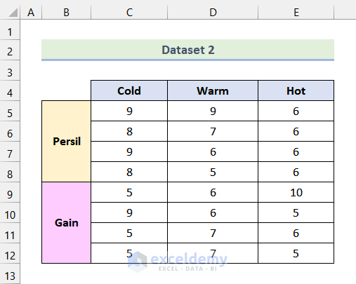
In the following dataset, we have the amount of dirt removed by 2 different brands of detergents named Persil and Gain and in 3 different temperatures of water. Here, the amount of dirt removed is dependent on 2 factors. They are the brand of the detergents and the temperature of the water. For this reason, we will use the two way ANOVA here.

Steps:

Firstly, follow the steps mentioned in Step 01 of the previous method if the Analysis ToolPak Add-in is not available.
Following that, go to the Data tab from the Ribbon.
Then, click on the Data Analysis option.

Consequently, the Data Analysis dialogue box will open as shown in the image given below.

Now, from the Data Analysis dialogue box, select the Anova: Two-Factor With Replication option.
Then, click OK.

Following that, from the Anova: Two-Factor With Replication dialogue box, click on the Input Range box.
After that, select the dataset as marked in the following image.
Subsequently, in the Rows per sample box, enter 4. Because in our dataset we have 4 samples for each brand of detergents.
Now, in the Alpha box enter the value 0.05 which is the standard value of Alpha.

Next, click on the Output Range box,
Afterward, select the cell from where you want to display the output. In this case, we have selected cell B14.
Finally, click OK.

Congratulations! You have successfully done the two way ANOVA test. The outputs should look like the following image.

Practice Section

In the Excel Workbook, we have provided the practice section on the right side of the worksheets. Please do it by yourself.

Download Practice Workbook

Doing ANOVA.xlsx

Conclusion

Finally, we have come to the very end of our article. I truly hope that this article was able to guide you to do ANOVA in Excel. Please feel free to leave a comment if you have any queries or recommendations for improving the article’s quality. Happy learning!