The article will show you how to interpret ANOVA single factor results in Excel. The Analysis of Variance (Analysis of Variance), is a dedicated statistical model to find the differences in averages within one or multiple groups. Single-factor ANOVA is useful when a single variable in the dataset plays the key role. The purpose of this analysis is to find if the data significantly differs from the mean. The article will pave the way for you to show the procedures of interpreting the ANOVA single factor results step by step.
How to Interpret ANOVA Single Factor Results in Excel: Easy Steps
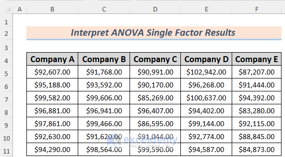
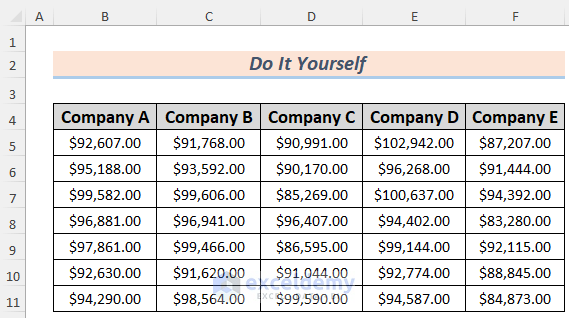
In the dataset, we have information about the yearly salaries of some employees in different companies. We will compare the salaries by the ANOVA single factor analysis in the following sections of this article.
Step 1: Initializing Data Analysis Toolpak
If you don’t have the Data Analysis Toolpak enabled in your Excel workbook, you need to do that first.
- Go to the File
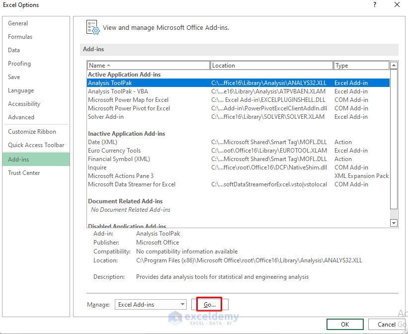
- After that, select the Options

- Next, select Add-ins >> Analysis Toolpak.
- Thereafter, select Excel Add-ins from the Manage section and click on Go.
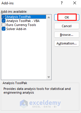
- After that, a dialog box will show up. Check Analysis Toolpak and click OK.
- This command will add the Data Analysis Toolpak in the Data Tab. Now select this Add-in.
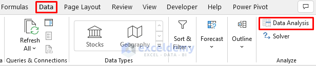
Step 2: Applying ANOVA Single Factor Analysis to the Dataset
We’ve set our necessary arrangement to analyze our data by the ANOVA Single Factor feature. Now let’s apply this to our data.
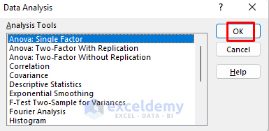
- After clicking on the Data Analysis Toolpak, the Data Analysis window will appear.
- Next, select Anova: Single Factor and click OK.
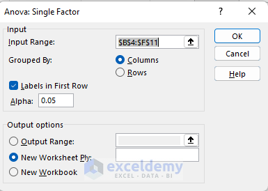
- Thereafter, insert the range of your dataset in the Input Range Our data remains in the B4:F11 range, so we put it.
- Make sure to check Labels in First Row.
- Next, choose a Significance value (Alpha, a). Here we insert 05 as the value of Alpha.
- After that, select the Output range according to your convenience. In my case, I selected New Worksheet to analyze the Output of this application.
The command will provide the ANOVA Single Factor Results in a new worksheet.
Step 3: Interpreting ANOVA Single Factor Results
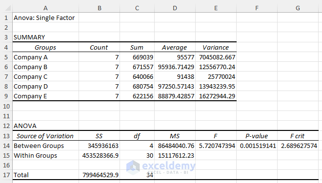
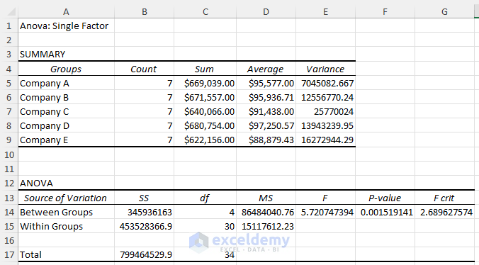
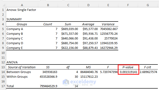
In this step, we will be interpreting the ANOVA Single Factor Results with the help of the values we get from the previous step. Let’s just convert the Sum and Average values to the Currency format for our convenience.
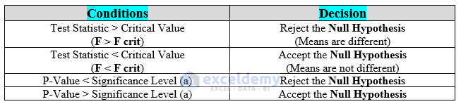
The following image shows the conditions for the acceptability or rejection situation of Null Hypothesis.
Parameters: ANOVA Analysis compares data with the means of various groups using various parameters. Let’s discuss them below.
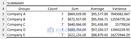
Average and Variance: From the Summary, we can see that the highest Average value and Variance are found for companies D and E respectively (97250.57 $ and 25770024).
Test Statistic (F) vs. Critical Value (F crit): In our Single Factor ANOVA analysis, the test statistic value (F) is 5.72 and the Critical Statistic value (F Crit) is 2.69. As F > F crit, the data model rejects the Null Hypothesis.
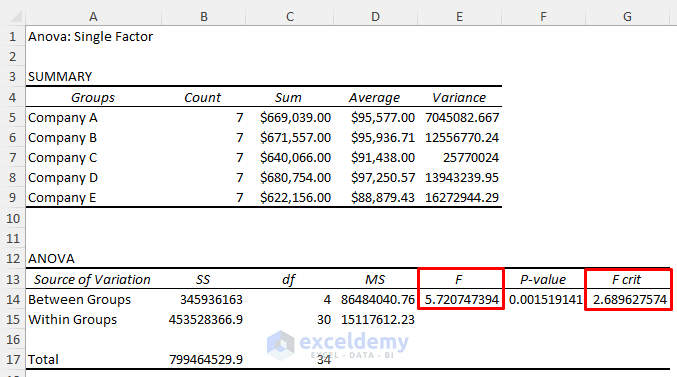
P-Value vs. Significance Level (Alpha or a): We also found that the P-Value is 0.0015 from the Single Factor interpretation which is smaller than the Significance Level (a = 0.05). So, we can surmise that the means are significantly different and reject the Null Hypothesis.
Thus you can interpret ANOVA Single Factor results in Excel using the Data Analysis Toolpak.
Read More: How to Interpret ANOVA Results in Excel
Practice Section
Here, I’m giving you the dataset of this article so that you can practice these methods on your own.
Download Practice Workbook
Conclusion
In the end, we can pull the bottom line by considering that you will learn the way of interpreting the ANOVA single factor results in Excel after reading this article. If you have any better suggestions or questions or feedback regarding this article, please share them in the comment box. This will help me enrich my upcoming articles.
Related Articles
- Nested ANOVA in Excel
- How to Make an ANOVA Table in Excel
- How to Calculate P Value in Excel ANOVA
- How to Perform Regression in Excel and Interpretation of ANOVA
- How to Graph ANOVA Results in Excel
<< Go Back to Anova in Excel | Excel for Statistics | Learn Excel
Get FREE Advanced Excel Exercises with Solutions!
