The fact that Microsoft Excel can only handle balancing designs in which each sample does have an equal amount of observations is among its most notable restrictions. From a technical standpoint, doing a Two-Way ANOVA with an asymmetrical structure is much more complicated and challenging, and you will require some statistical package to do this. As we are aware, ANOVA is used to determine the mean difference between groups that are larger than two. In this article, we will demonstrate the instructions to do two-way ANOVA in Excel.
What Is ANOVA?
ANOVA is a statistical analysis technique that divides methodical components from different variables to account for the apparent collective variation within a data set. When there are more than two groups, the difference among both may be determined using an ANOVA. When there are two classification factors and a continuous result, the difference can be determined using a two-way ANOVA. Although there are many different types of ANOVA, the main goal of this family of studies is to ascertain if variables are associated with an outcome variable.
A two-way ANOVA is performed as a statistical test to ascertain how two or more explanatory regression models would affect a continuous result variable.
ANOVA with two components is another name for it which is Analysis of Variance. Whenever there is one measurement parameter and two independent parameters referred to as determinants or primary effects we employ the approach. We require observations for each conceivable variation of the theoretical amounts in order to use this methodology.
Step 1: Enabling Data Analysis ToolPak to Perform Two way ANOVA in Excel
Excel’s Data Analysis feature gives the ability to ask questions about data in normal language rather than needing to create laborious algorithms. But by default Excel disables this ToolPak from the ribbon. To enable this feature we need to follow the following steps.
- To begin with, go to the File tab from the ribbon.
- This will take you backstage of the Excel spreadsheet.
- Further, in the bottom left corner, click on the Options menu.

- Excel Options dialog box will appear.
- Next, go to Add-ins.
- Furthermore, from the Add-ins group, click on Analysis ToolPak.
- After that, in the Manage drop-down menu, select Excel Add-ins.
- Consequently, click on the Go… button.

- This will display the Add-ins dialog box.
- Now, checkmark the Analysis ToolPak option from Add-ins available options list.
- Finally, click on the OK button to finish the procedure.

Step 2: Creating Two-Way Table
We must gather information on the qualitative predictor variables at varying configurations of 2 autonomous descriptive analyses in order to apply the Two-Way ANOVA analysis. Firstly, we need to arrange our dataset appropriately in order to do a two-factor analysis of variance in Excel.
- In the first place, we take three items in column B, which are the sample rows to perform the two-way ANOVA.
- Afterward, put the percentage of the supplier sequentially in columns C, D and E.

Step 3: Use Data Analysis Tool to Do Two way ANOVA
The Data Analysis ToolPak can help to develop intricate statistical or technical studies faster and with fewer steps.
- Firstly, go to the Data tab from the ribbon.
- Secondly, click on the Data Analysis tool under the Analysis category.
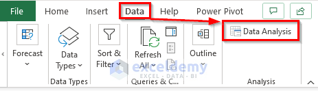
- Thus, the Data Analysis dialog box will appear.
- Now, from the Analysis Tools options, select Anova: Two-Factor With Replication.
- Consequently, click OK.

- Therefore, the Anova: Two-Factor With Replication dialog will display.
- Now, click on the upper arrow icon shown in the screenshot below to set the Input Range.

- Further, a tint dialog will pop up where we set the range. In our case, we take the range $B$4:$E$10.
- Then, press the Enter key on your keyboard.

- Additionally, we can see that the range is now set in the Input Range field.
- As we have three items, we take three in the Rows per sample box.
- Lastly, click on the OK button to complete the process.

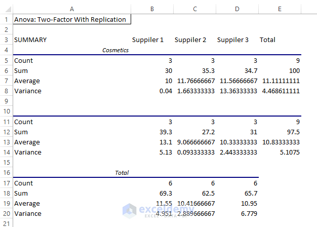
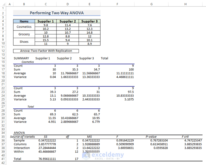
Step 4: Summary Statistics of ANOVA in Excel
The patterns for the essential includes and the general average for the two aspects vary. Due to the greater disparity here between providers for the middle item. Suppliers’ average is greater compared to the other suppliers. This average analysis may help us anticipate the results of the two-way ANOVA under the atheist position that the variables have no influence.
Read More: How to Interpret Two-Way ANOVA Results in Excel
Step 5: Hypotheses Test Result of Two way ANOVA
We cannot simply assert that one supplier type causes a greater tear intensity since the P-value for the association is so low. The alternative hypothesis supports what we could have anticipated based on the analysis of average values: The type of box determines how the various cassettes work.
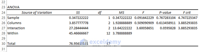
This is the final output after performing the two-way ANOVA analysis in that specific data in an Excel spreadsheet.
Read More: Two Way ANOVA in Excel with Unequal Sample Size
Things to Keep in Mind
A #NUM error often happens if each combination of the component groups does not contain the same number of sample rows in the ANOVA dialog.
Download Practice Workbook
You can download the workbook and practice with them.
Conclusion
The above procedures will assist in how to do two way ANOVA in Excel. Hope this will help you! Please let us know in the comment section if you have any questions, suggestions, or feedback.
Related Articles
- How to Make an ANOVA Table in Excel
- How to Use Two Factor ANOVA with Replication in Excel
- How to Do Repeated Measures ANOVA in Excel
- How to Apply Rows Per Sample ANOVA in Excel
- Randomized Block Design ANOVA in Excel
- How to Do One Way ANOVA in Excel
- How to Use ANOVA Two Factor Without Replication in Excel
<< Go Back to Anova in Excel | Excel for Statistics | Learn Excel
Get FREE Advanced Excel Exercises with Solutions!
