In this article, we will do repeated measures ANOVA in Excel. We can perform different types of data analysis with the help of Microsoft Excel. ANOVA stands for Analysis of Variance. In repeated measures ANOVA, we compare the means across one or more variables based on repeated observations. It determines the significant difference among the means of three or more groups. Today, we will show step-by-step procedures. Using these steps, you can efficiently perform repeated measures ANOVA in Excel.
How to Do Repeated Measures ANOVA in Excel: Easy Steps
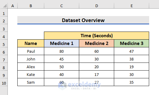
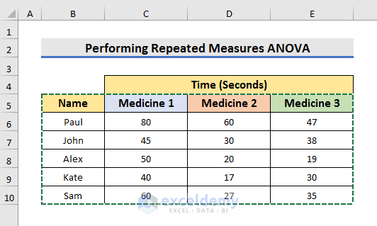
To explain the steps, we will use a dataset that contains information about the reaction time of 3 medicines in 5 patients. Here, the reaction time for medicines was measured 3 times for each patient. So, we will apply repeated measures ANOVA to check if the mean reaction time differs among drugs. Unfortunately, there is no default option or function to do the repeated measures ANOVA. But we can use the ‘Anova: Two-Factor Without Replication’ option to get the repeated measures ANOVA.
STEP 1: Open Data Analysis ToolPak
- In the first place, we need to open the Data Analysis ToolPak.
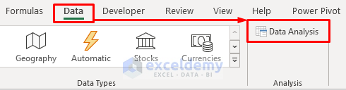
- To do that, go to the Data tab and select the Data Analysis option. It will open the Data Analysis dialog box.
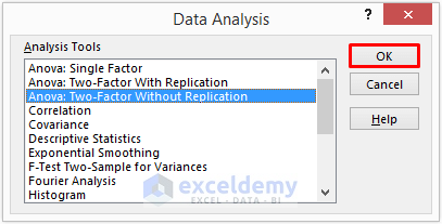
- In the Data Analysis dialog box, select ‘Anova: Two-Factor Without Replication’ and click OK to proceed.
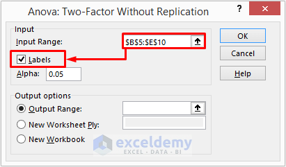
- It will open the Anova: Two-Factor Without Replication dialog box. You need to insert the Input Range and Output Range in that box.
STEP 2: Select Input Range
- Secondly, we will select the input range.
- For that purpose, click on the Input Range box and make sure the cursor is blinking.
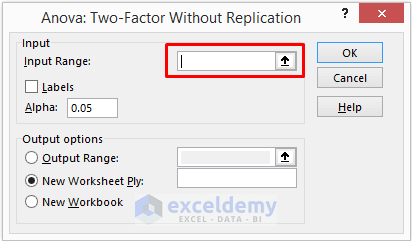
- After that, select the desired input range with the headers. Here, we have selected the range B5:E10.
- Also, check the Labels.
STEP 3: Choose Output Range
- Thirdly, you need to choose the output range. It’s the range where the results will appear.
- Now, select Output Range and click on the box of the Output Range.
- Make sure the cursor is blinking.
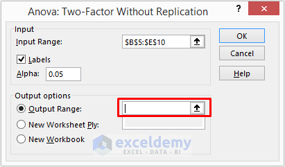
- In the following step, select the cell from where you want to start showing the results.
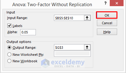
- We have selected Cell G3 here.
- Similarly, you can also display them on a new sheet by selecting the ‘New Worksheet Ply’ option.
- Click OK to move forward.
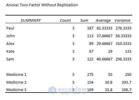
STEP 4: Review Summary Table
- After clicking OK, the summary table will appear on the sheet.
- You can see each patient and medicine’s sum, average, and variance separately.
STEP 5: Evaluate Repeated Measures ANOVA
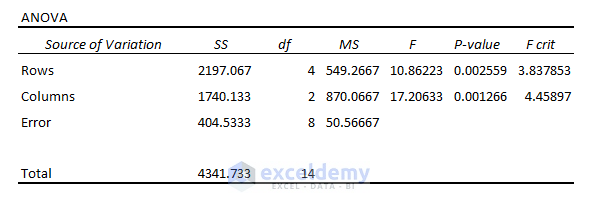
- After watching the summary table, if you scroll down you can see the ANOVA table also.
- Here, you will find the value of SS, df, MS, F, P-value, and F crit for rows and columns.
STEP 6: Analyze Results
- In our case, we will look for the F test-statistic value and the corresponding P–value for Columns.
- Because the value of the columns will tell us if the reaction time of the medicines differs.
- From the table, we can say that the F test-statistic value is 17.20633 which is less than the F critical value of 4.45897.
- Also, the corresponding P–value is 0.001266.
- The P–value is less than 0.05. That’s why we can reject the null hypothesis.
- In conclusion, we can say that there is a significant difference in the reaction time of the medicines.

Read More: How to Interpret ANOVA Results in Excel
Download Practice Book
You can download the practice book from here.
Conclusion
In this article, we have discussed step-by-step procedures to do repeated measures ANOVA in Excel. I hope this article will help you to perform your tasks efficiently. Furthermore, we have also added the practice book at the beginning of the article. To test your skills, you can download it to exercise. Lastly, if you have any suggestions or queries, feel free to ask in the comment section below.
Related Articles
- How to Do Two Way ANOVA in Excel
- How to Make an ANOVA Table in Excel
- How to Apply Rows Per Sample ANOVA in Excel
- Randomized Block Design ANOVA in Excel
- How to Do One Way ANOVA in Excel
- Two Way ANOVA in Excel with Unequal Sample Size
- How to Use Two Factor ANOVA with Replication in Excel
- How to Interpret Two-Way ANOVA Results in Excel
<< Go Back to Anova in Excel | Excel for Statistics | Learn Excel
Get FREE Advanced Excel Exercises with Solutions!
