Randomized Block Design ANOVA in Excel (with Easy Steps)

What Is ANOVA?

ANOVA (Analysis of Variance) summary tables are important to understand whether the groups significantly differ from each other. Basically, ANOVA finds the impact of different hypotheses in a treatment.

How to Do Randomized Block Design ANOVA in Excel: 2 Steps

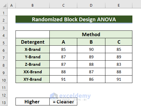
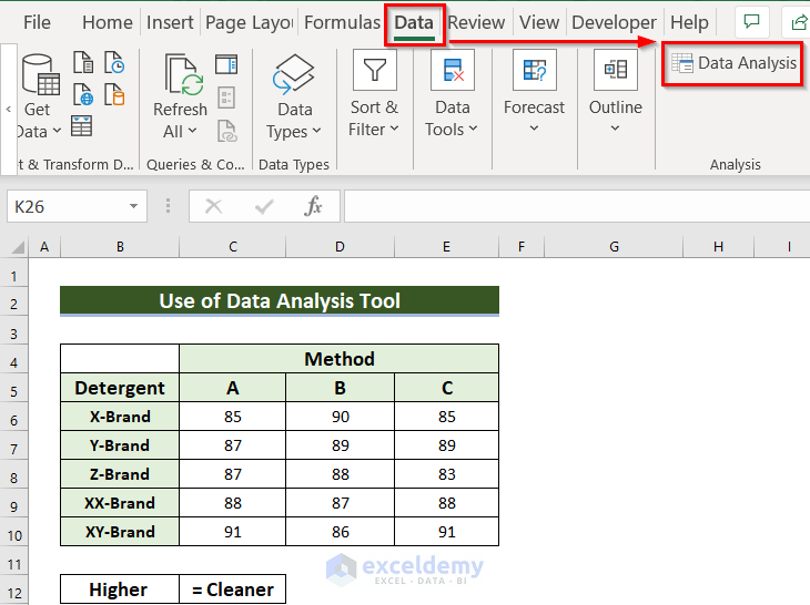
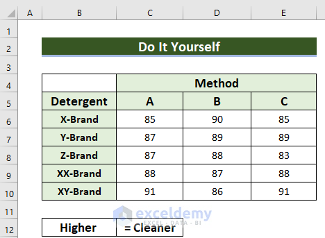
We’ll use sample data with 4 columns to find out if there are any differences among detergents. The higher marks denote more cleanness.

Check whether your Excel Data tab contains Data Analysis. If the Data Analysis ToolPak exists, go to Step 2.

Here, I’m going to use Microsoft 365 to do randomized block design ANOVA in Excel.

Step 1 – Inserting the Data Analysis ToolPak for Randomized Block Design ANOVA

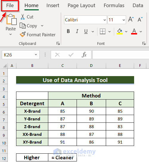
Go to the File tab.

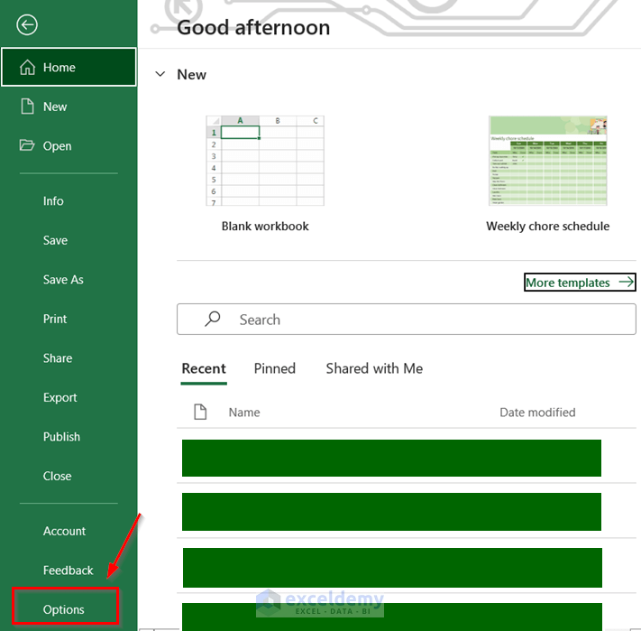
Choose Options.

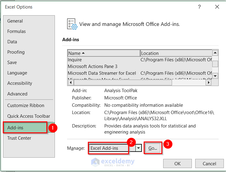
A dialog box named Excel Options will appear.

Go to the Add-ins command.
Choose Excel Add-ins in the Manage: box.
Press the Go button.

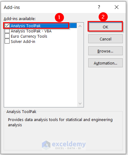
Another dialog box named Add-ins will appear.

Click on the Analysis ToolPak.
Press OK to get the changes.
Close the Options window.

You’ll get a new option named Data Analysis under the Data tab.

Step 2 – Doing Randomized Block Design ANOVA in Excel

From the Data tab, select Data Analysis.

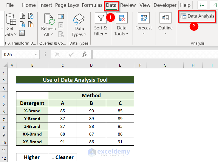
A dialog box named Data Analysis will appear.

Select Anova: Two-Factor Without Replication and click on OK.

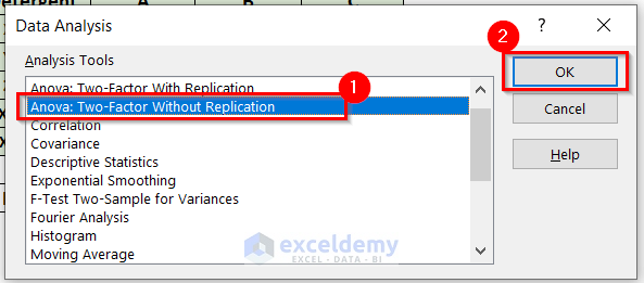
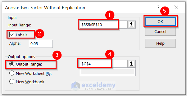
A new dialog box named Anova: Two-Factor Without Replication will appear.

Select the data range in the Input Range: box for which you want to do the randomized block design ANOVA. We have selected the range B5:E10.
Mark the Labels option.

Alpha is the significance value.

Choose the cell in the Output Range: box where you want to see the result. We have chosen the G4 cell.
Press OK to get the result.

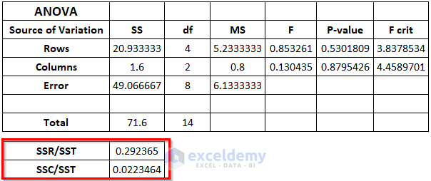
You will get the following output.

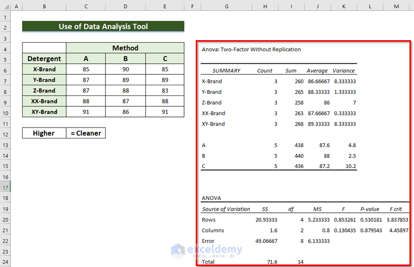
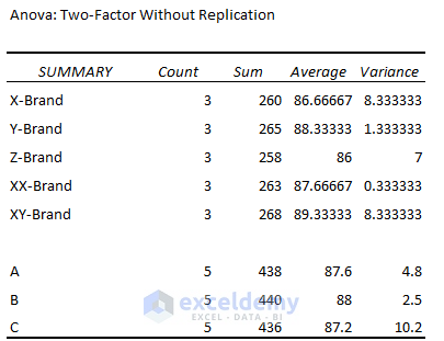
The Anova: Two-Factor Without Replication calculates the Count, Sum, Average, and Variance. All the detergent types have those outputs, including each method. The COUNT, SUM, and AVERAGE function works both horizontally (for Brands) and vertically (for Methods).

Higher numbers denote higher cleanliness. Variance denotes the changing rate with the brand and methods.

Here is the ANOVA summary table. Rows denote blocks and Columns denote treatments.

We will consider the null hypothesis when the P-value exceeds the significance value. If the F value is less than the F critical value then there will be no difference between them, which is the null hypothesis. So, there is no difference between those detergents or methods.

Let’s see the first three terms. Here, SS denotes the sum of squares, df denotes the degree of freedom and MS denotes mean squares.

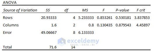
If we divide the sum square of rows by the total sum square, it returns 0.29. This means around 29% variance can be explained by the impact of detergent brands (blocks). When we divide the sum square of columns by the total sum square, it returns 0.022. This means around 2.2% variance can be explained by the impact of methods.