A histogram is one kind of graph which we use to show frequency distribution within some prespecified ranges. These data ranges are called ‘bins’. The histogram chart shows how many data points belong to each of these bins. This article will illustrate how to plot a histogram using cumulative data in Excel with easy steps and proper illustrations.
How to Plot Cumulative Histogram in Excel: Step-by-Step Procedures
1st Step: Collect Data
The very first step is- to collect your data and gather them in an Excel spreadsheet.
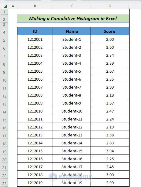
- Here we have collected 55 students’ grade points data (CGPA).
2nd Step: Find Maximum and Minimum Values in the Data
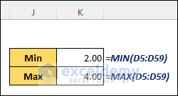
- To find the maximum value in the range D5:D59, use the MAX function.
=MAX(D5:D59)- To find the minimum value in this range, use the MIN function.
=MIN(D5:D59)- Here, we have found the maximum and minimum values (2.00 and 4.00)
3rd Step: Add a New Column for Bins
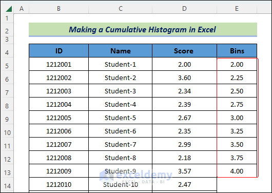
The 3rd step is creating suitable bins. This is up to you. You can create bins with any width.
- Here, we have specified 0.25 as the width.
- You can use the following common formula and drag it down until you reach the maximum value 4.00.
- Here, we have first input the minimum value in cell E5 and then used the following formula.
=IF(E6>4,"",E5+0.25)- The output will be as follows.
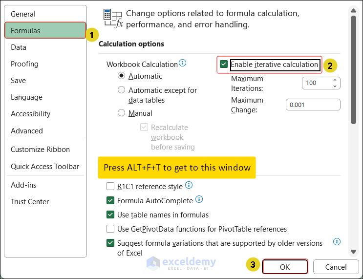
This is an iterative formula. Iterative formulas cause circular reference issues. To make this type of formula work, press ALT+F+T and go to the Formulas section, there, mark the “Enable iterative calculation” box and press OK.
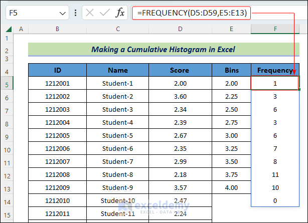
4th Step: Employ FREQUENCY Function of Excel to Get the Frequencies That Belong to Each Bin
The FREQUENCY function returns the number of occurrences of a value within a bin_range. It returns one more element than the specified bins_array, in our case, we will delete that.
- The common formula is:
- Write the following formula in cell F5.
=FREQUENCY(D5:D59,E5:E13)Here, D5:D13 is the data_array and E5:E13 is the bins_array which stands for the range of values.
- Now, copy the cells F5:F14 and paste the values only, in the same place F5:F14.
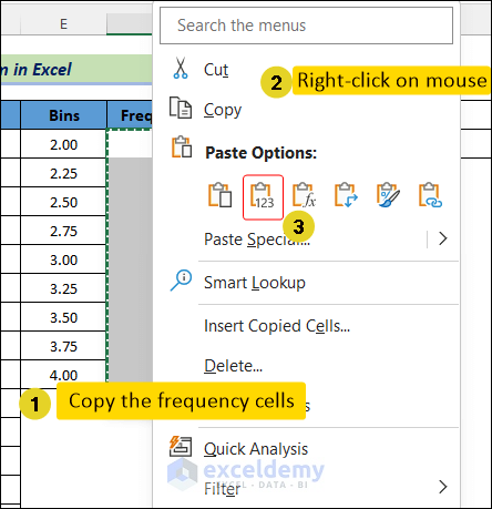
- Now, delete the last 0.

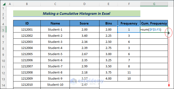
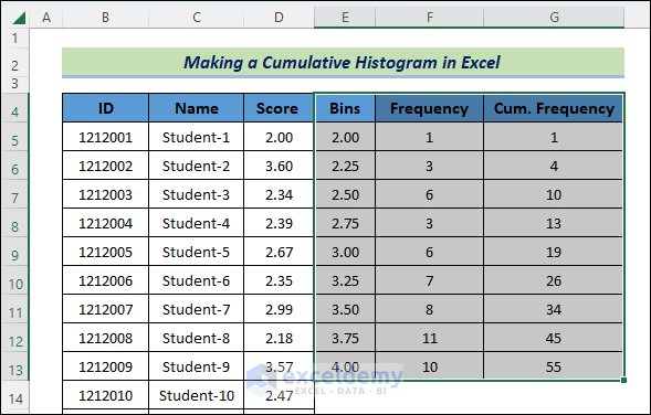
5th Step: Calculate Cumulative Frequency
- Now, add a new column named Cum. Frequency and apply the following formula in cell G5.
=SUM($F$5:F5)- The common formula is:
- Now, drag the fill handle icon to copy the formula downside.
Last Step: Plot Cumulative Histogram from Recommended Charts
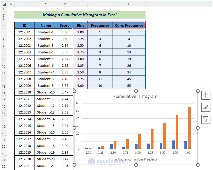
- Now, select the whole range that contains Bins, Frequency, and Cum. Frequency columns, E4:G13.
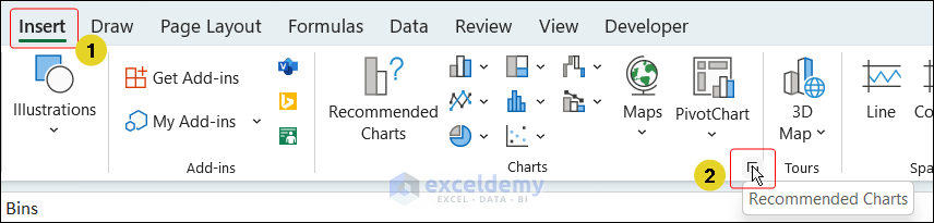
- Then go to the Insert tab.
- From the Charts group, click on the tiny Recommended Charts icon.
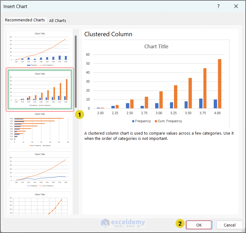
- From the Insert Chart window, select the 2nd chart type and press OK.
Here the procedure ends. Look at the following image, we have drawn the cumulative histogram successfully.
Read More: How to Create Probability Histogram in Excel
Download Practice Workbook
Conclusion
I hope this brief discussion will help in plotting a cumulative histogram in Excel. If you have any queries, please let us know in the comment box. Visit us and enjoy Excelling!
Related Articles
- How to Create a Histogram with Bell Curve in Excel
- How to Plot Histogram with Unequal Class Intervals in Excel
- How to Add Vertical Line to Histogram in Excel
- Stock Return Frequency Distributions and Histograms in Excel
- How to Create Histogram in Excel Using VBA
<< Go Back to Excel Histogram | Excel Charts | Learn Excel
Get FREE Advanced Excel Exercises with Solutions!
