The Confidence Interval is an important indicator of the limitations of estimates in a set of data. It is important to measure if enough simulations are done in observation, it helps to identify the validity of a curve, and helps determine if a change in any simulation is significant or not. And adding the error bars in a chart of confidence intervals helps us to identify them and visualize their significance easily with the graphs. In this article, we will describe the method to add confidence interval error bars in Excel charts in detail.
What Is Confidence Interval?
Before starting the calculation, we must understand the confidence interval first. According to statistics, it is basically a probability of a specific parameter that falls between a couple of values. Confidence interval measures the level of certainty of uncertainty in a trial process.
Now, in the case of proportion, the confidence interval provides a range of values that contains a proportion of the population with a level of confidence in a specific sample test. The values show the confidence interval proportion for both high and low estimations.
To calculate the confidence interval for proportion, we have to use this formula.

Here,
x̅ = Mean of the population
z = Confidence level value
s = Standard deviation
n = Sample size
What Are Error Bars in Excel?
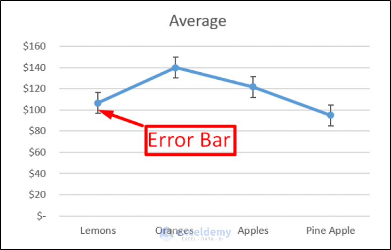
Error Bar is a graphical representation. It describes the variability of data and represents the error or uncertainty in a given data. It can give a general idea about the data.
Error bars in your charts can help you quickly see ranges of error and standard deviations. They can be displayed as a standard error amount, a standard deviation, or a percentage on all data points in a data series. You can customize the mistake amounts displayed by entering new values. For example, in the results of a scientific experiment like the following, you can show a 10% positive and negative error amount.
We can use error bars in the two-dimensional area of column, bar, XY (scatter), line, and bubble charts. Also, we can display error bars for x and y values in scatter and bubble charts.
How to Add Confidence Interval Error Bars in Excel: Step-by-Step Procedure
To add confidence interval error bars in Excel, we first need to find out the confidence intervals or confidence interval errors using either the function or the formula we discussed above. In the steps, we will be calculating the error values manually. You can also use the CONFIDENCE function to find almost the same values.
Also, we will be focusing on determining the values at a 90% confidence interval. Although the process is the same for any number of confidence levels, the z value changes with them. So using the proper z value is important. For a 90% confidence interval, the z score would be approximately 1.64. If you want to find out individual z-score values depending on your confidence level in Excel, click here to see how to calculate z-score in Excel.
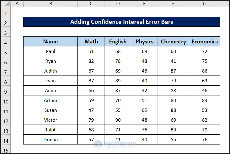
The dataset for today’s example would be as follows.
We will use the following steps to calculate and add confidence interval error bars in Excel.
Step 1: Calculate Mean for Each Column
In addition to the data in the dataset, we need to find some more values from them in order to find confidence interval errors and add the bars in Excel. With this in mind, let’s prepare some cells and extend the dataset first.

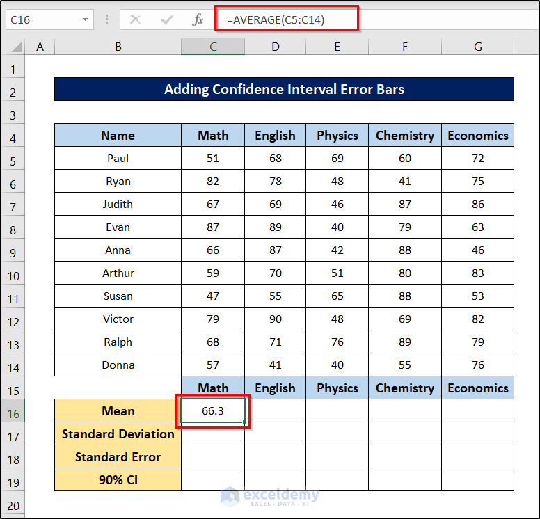
We need to use the AVERAGE function to calculate the average or mean for each subject here. With this intention, follow these steps.
- First, select cell C16.
- Then write down the following formula.
=AVERAGE(C5:C14)
- After that, press Enter.
- Finally, select the cell again and click and drag the fill handle icon to the right to fill the rest of the cells with their respective references.
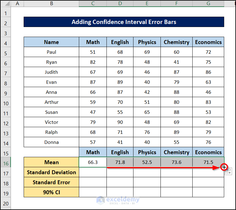
This is how we find the mean for each subject in this dataset.
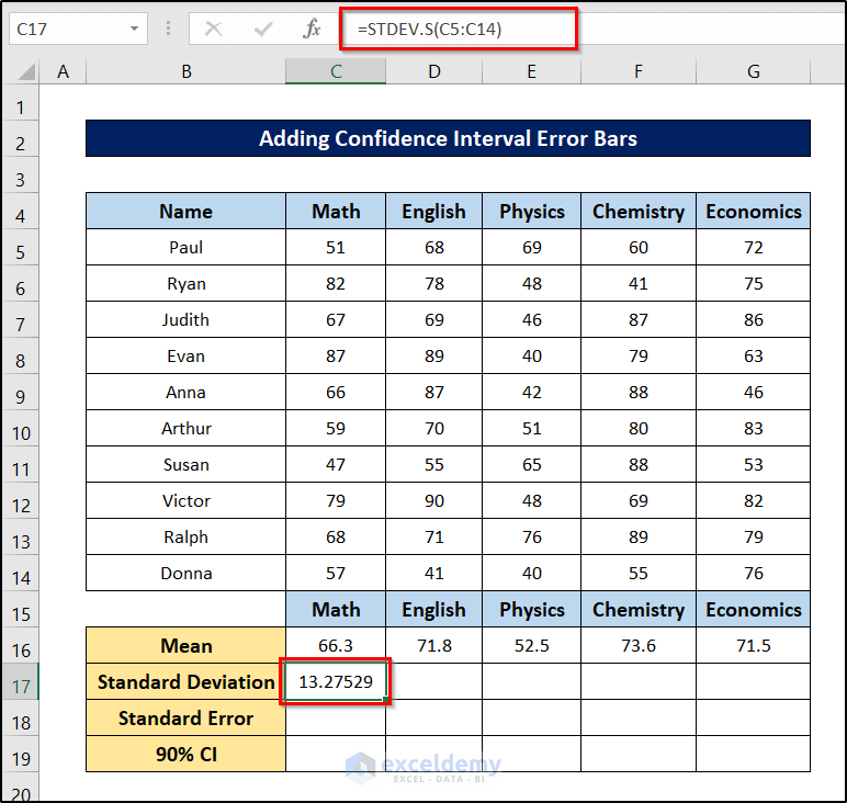
Step 2: Compute Standard Deviations
Now it is time to find the standard deviations here. To find the standard deviations in Excel, we use the STDEV.S function. You can also use the STDEV function for the same purpose. But it is more compatible with the older versions of Excel. Both of these functions take several arguments and return the standard deviation ignoring logical and text values.
To find the standard deviations in this dataset, you can follow these steps.
- First, select cell C17.
- Now write down the following formula.
=STDEV.S(C5:C14)
- Then press Enter.
- After that, select the cell again. Finally, select the cell again and click and drag the fill handle to the right of the row to fill the rest of the cells with the formula.
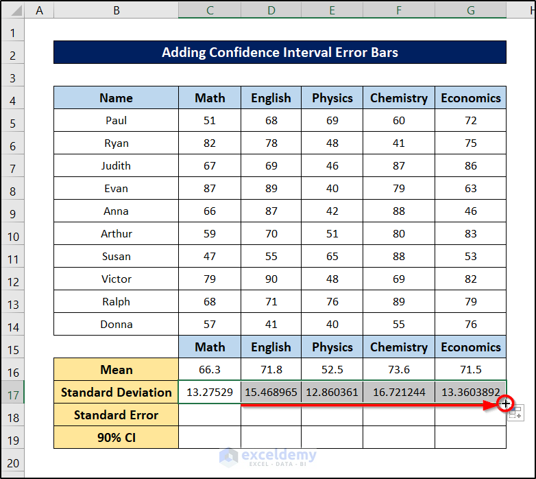
Thus we find the standard deviation of marks for each subject that we will use later on to add confidence interval error bars in Excel.
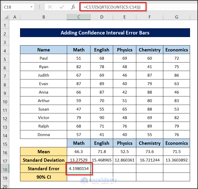
Step 3: Calculate Standard Errors
We will now find the standard error values from the standard deviations. Because of that, we need the COUNT and SQRT functions. The COUNT function takes a number of arguments or an array and returns the total number of arguments or members in the array. Meanwhile, the SQRT function takes an argument and returns the root of the same.
To find the standard error of this dataset, you can follow these steps.
- First, select cell C18.
- Then write down the following formula.
=C17/(SQRT(COUNT(C5:C14)))
- After that, press Enter.
- Finally, select the cell again and click and drag the fill handle icon to the right of the row to replicate the formula for the rest of the cells.
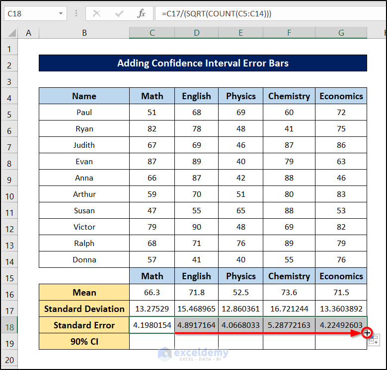
As a result, the standard error value calculations are now complete.
Step 4: Calculate Confidence Intervals
Next, we will calculate the confidence intervals with a confidence level of 90%. For that, the z score would be 1.64. The formula for the confidence interval is the z score times the standard error. So we are gonna use a simple multiplication formula here to find that.
- First, select cell C19.
- Then write down the following formula in it.
=1.64*C18
- After that, press Enter.
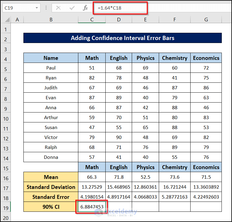
- Finally, select the cell again and click and drag the fill handle icon to the right of the row to fill the rest of the cells with the formula with their respective references.
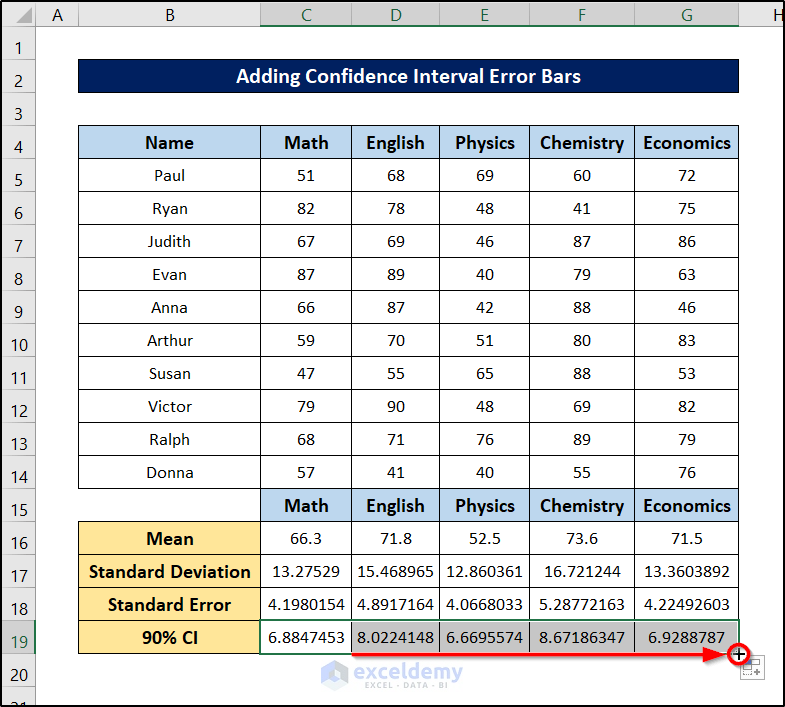
As a consequence, we will have the 90% confidence interval values for each subject of which we will plot error bars later on in Excel.
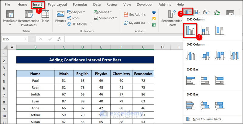
Step 5: Insert Column Chart
To add confidence interval error bars, we need to first plot a chart in Excel. We are opting to go for a bar plot for our dataset. You can also choose any other chart you want.
To plot a bar at this point, follow these steps.
- First, select the range you want to plot the data from. In this case, it is the mean values with the subjects. So we have chosen the range B15:G16.
- Then go to the Insert tab on your ribbon.
- After that, select the Insert Column or Bar Chart icon from the Charts group section.
- Now select Clustered Column from the drop-down menu.
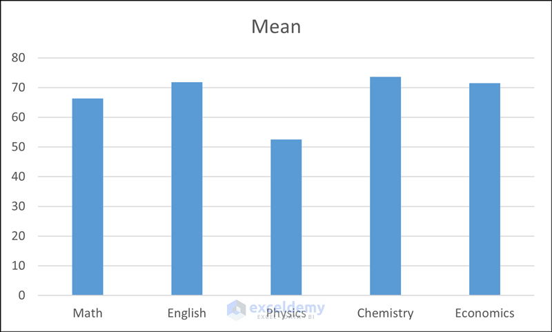
- Once you have done that, you will have the chart pop up on the spreadsheet like the following figure.
Step 6: Switch Rows/Columns
We now need to switch the rows and columns in the graph for later actions. Subjects are what we need in the horizontal axis instead of the mean values. This is just a preparation for adding confidence interval error bars for this Excel chart. For that, follow these steps.
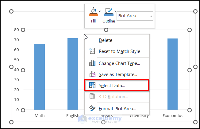
- First, right-click on anywhere on the graph.
- Then select the Select Data option from the context menu.
- As a result, the Select Data Source box will open up.
- Now select the Switch Row/Column button here.
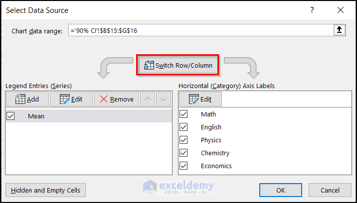
- After that, click on OK.
The chart will now look something like this.

You can now keep on going to the following steps.
Step 7: Add Error Bar to Column
Once we have plotted and prepared the chart, we can now continue to add error bars. In this case, we will add confidence interval error bars in the Excel chart. With this in mind, you can follow these steps to add confidence interval error bars within Excel.
- First, click on a bar on the chart.
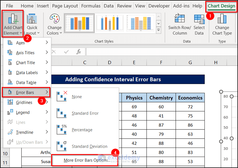
- Then you will notice the Chart Design tab appear on your ribbon. Select it.
- After that, select the Add Chart Element option from the Chart Layouts group section.
- Then hover your mouse over the Error Bars from the drop-down menu.
- Now click on the More Error Bar Options.
- As a result, the Format Error Bars window will appear on the right of the spreadsheet.
- Here, you will find the Error Amount under Error Bar Options.
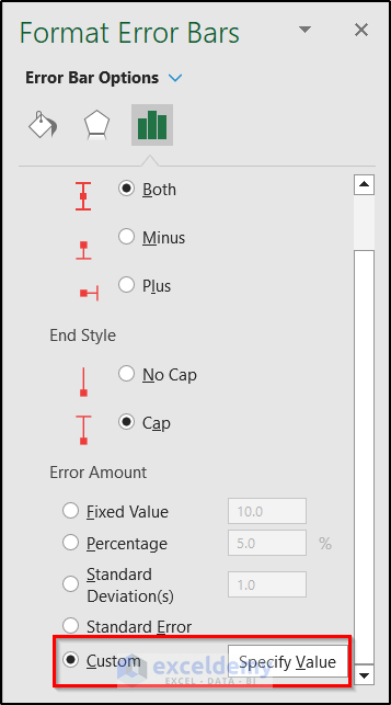
- Now select Custom as the Error Amount option here.
- Then click on Specify Value.
- In the next box, put both the Positive Error Value and Negative Error Value as the 90% confidence interval values which we indicate as follows (“90% Ci” is the spreadsheet name).
='90% CI'!$C$19
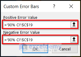
- Then click on OK.
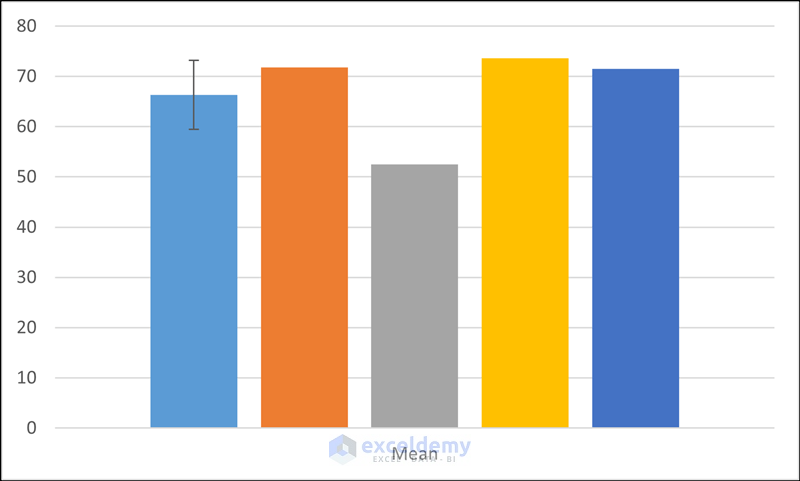
Thus you will have the confidence interval error bar of the column on the Excel chart.
Step 8: Repeat for All Columns
We have added a confidence interval error bar in a column in the previous step. Now for the rest of the columns, we can repeat the process and find all of the confidence interval error bars on the Excel chart.
Just keep in mind that you have to insert the corresponding confidence interval values to their columns. Unfortunately, we have to go through the process manually for each column. Nevertheless, the idea and process are the same.
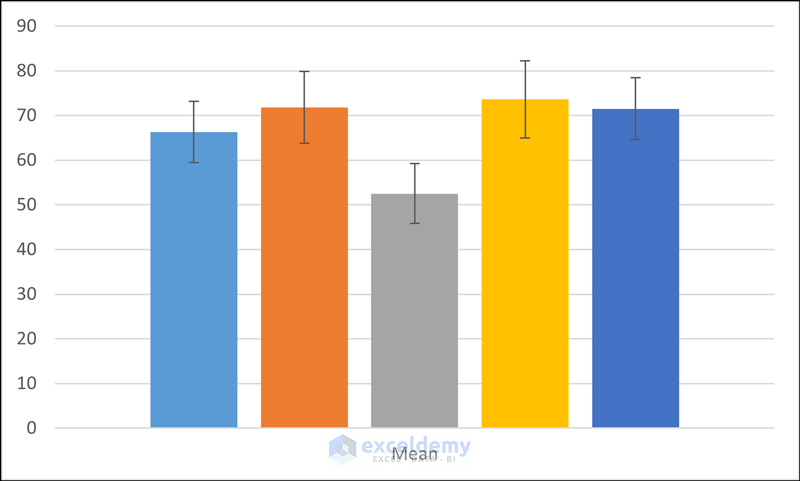
Once you have repeated step 7 for all the columns, the figure will look something like this.
Step 9: Modify Chart to Make It More Presentable
Even though adding confidence interval error bars is complete within Excel, it may not be the prettiest or most visually pleasing graph. Now you are in your own space to modify it as you want.
For our case, we have added borders, legends, and the chart title, and made the error bars thicker to make it look more presentable.

Finally, the confidence interval error bars at 90% confidence for the average marks of students at different subjects is now complete with the help of Excel.
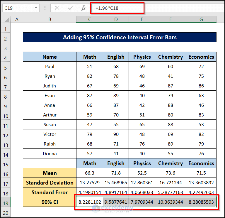
How to Add 95 Percent Confidence Interval Error Bars in Excel
Adding 95% confidence interval error bars is the same as adding 90% confidence interval error bars in Excel. The only difference is in the row values of confidence intervals. For a 95% confidence interval, the z-score is 1.96. So we have to adjust it accordingly.
- For a 95% confidence interval value, follow steps 1-3 from the previous section. Then on the final row, put in the following formula and fill it out.
=1.96*C18
- Now you can insert the bar plot for the range B15:G16 and switch the rows/columns.
- Then add an error bar by going to the Chart Design tab, and selecting Add Chart Elements. And then select Error Bars into More Error Bar Options.
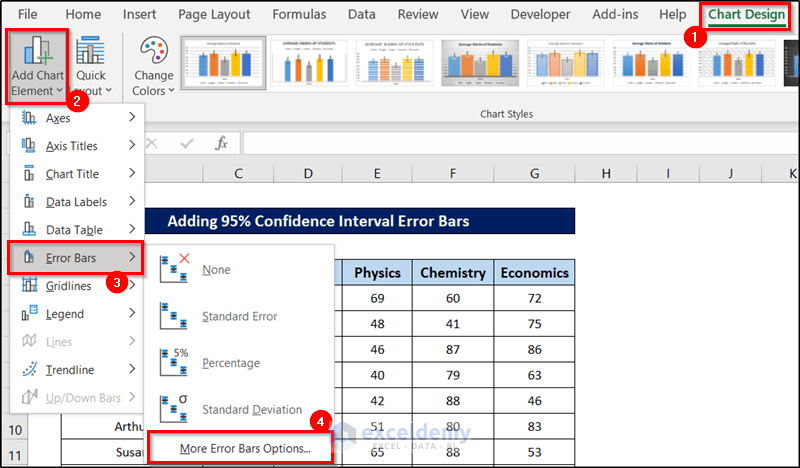
- On the right of the spreadsheet, you will find the Format Error Bars tab where select the Custom option as shown in the figure.
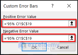
- Upon clicking on the Specify Value, as the box appears to insert a number, select the 95% confidence interval values this time.
='95% CI'!$C$19
- As a result, you will have the error bar appear on the selected column.

- Now repeat this for all the columns and you will have all the error bars at a 95% confidence interval in Excel.

How to Add Individual Error Bars in Excel
Now let’s suppose, we have the following bar plot ready at our disposal.

If you want to add an individual error bar on the chart in Excel, you need to select that column and then insert the error bar. This is the same as the one described in the previous two sections.
Steps:
- First, select the column, or point (for other types of charts) where you want to insert the individual error bar.
- Then go to the Chart Design tab on your ribbon.
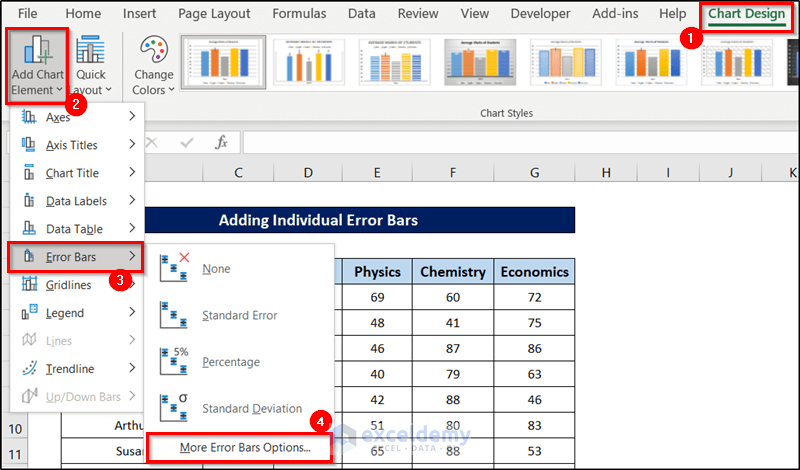
- After that, select Add Chart Elements from the Chart Layout group section.
- Then from the drop-down list, select Error Bars and More Error Bars Options.
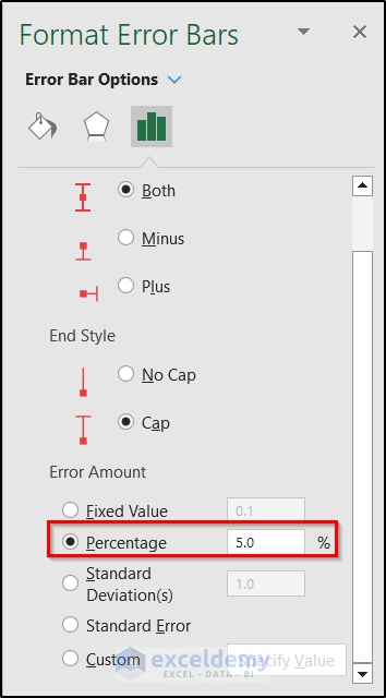
- Now find your preferred error amount to show in the bar under the Error Amount you can find on the Format Error Bars window on the left of the spreadsheet. Here, we have chosen Percentage as the error bar.
Once you have done that, you will find an error bar appearing on the selected column in Excel.

💬 Things to Remember
- You can only add individual error bars for specific measurements (e.g. percentage)
- Make sure to use the correct z-score while calculating the confidence interval from standard error.
Download Practice Workbook
Before we dive into the explanation, you can download the workbook used for the demonstration from the link below.
Conclusion
So that is all about confidence interval error bars in Excel. Hopefully, you have grasped the idea and can use it in practice for the dataset as well as your unique case. I hope you found this guide helpful and informative. If you have any questions or suggestions, let us know in the comments below.
Related Articles
- How to Calculate Confidence Interval Without Standard Deviation in Excel
- How to Calculate P-Value from Confidence Interval in Excel
- Excel Confidence Interval for Difference in Means
- How to Calculate Confidence Interval Proportion in Excel
- How to Calculate Population Proportion in Excel
- How to Calculate Confidence Interval for Population Mean in Excel
<< Go Back to Confidence Interval Excel | Excel for Statistics | Learn Excel
Get FREE Advanced Excel Exercises with Solutions!
