How to Use SQRT Function in Excel

In Mathematics and Trigonometry, we frequently need to know the square root of a number. The square root of an integer is a value that equals the number when multiplied by itself. MS Excel 2010 was the first to introduce the feature. The image below is a synopsis of the text, showing a few examples of how to use the SQRT function in Excel.

In the following sections of this tutorial, you’ll learn more about the methods and other functions that you’ll need to use the SQRT function correctly. In addition to the SQRT function, we’ve discussed some different techniques to find the square root and also the nth root of a number.

By the end of this article, you will have a clear understanding of how to utilize the SQRT function in Excel to solve complex mathematical problems, perform data analysis, and gain valuable insights. Whether you need to calculate the standard deviation of a dataset, analyze trends, or make data-driven decisions, mastering the SQRT function will undoubtedly empower you to work more efficiently and accurately.

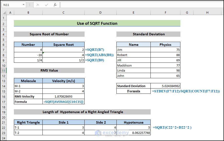
Below is an overview image of how to use the SQRT function in Excel.

Introduction to the SQRT Function

Function Objective:

The SQRT function in Excel returns the square root of a number.

Syntax:

=SQRT(number)

Arguments Explanation:

Return Parameter: The Excel SQRT function returns the square root of a positive number like for number 4 it returns the value 2.

How to Use SQRT Function in Excel: 7 Suitable Examples

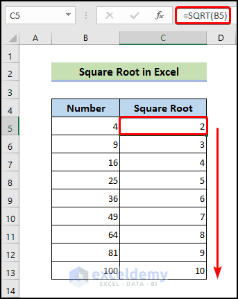
In this section, we will demonstrate 7 suitable examples to show the use of the SQRT function. This section provides extensive details on these examples. You should learn and apply these to improve your thinking capability and Excel knowledge. We use the Microsoft Office 365 version here, but you can utilize any other version according to your preference.

1. Basic Use of SQRT Function in Excel

The simplest way to compute square root in Excel is to use the function that was dedicated specifically for this purpose. The SQRT function returns the square root of a single argument (which could be a number or a reference to a number).

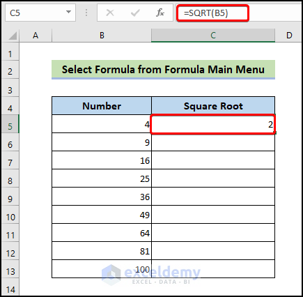
• Firstly, to calculate the square root, we have to type the following formula.

• Then, press Enter.
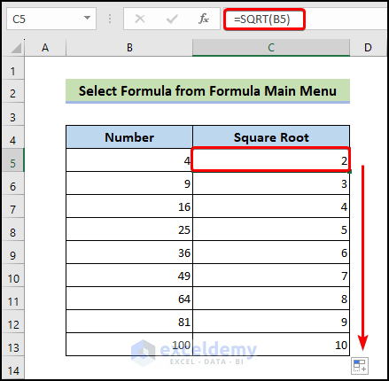
• Then, drag the Fill Handle icon to fill the other cells with the formulas.
• Therefore, you will get the following square root.

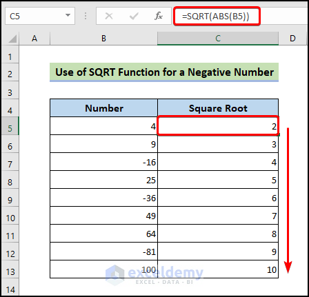
2. Apply the SQRT Function in Excel for a Negative Number

While this function works well with positive numbers, it will return a #NUM error if you give it a negative number. The following image shows what happens when we use the SQRT function. For positive numbers, we get the square root, but for negative numbers, we get a #NUM error.

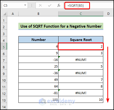
This is understandable because a negative number does not have a square root in mathematics. Even if a number is negative, multiplying it by itself produces a positive result.

If you still want to get the square root of a negative number (assuming it was a positive), you’ll need to convert it to a positive number first and then find the square root. You can combine the SQRT function with the ABS function to calculate the square root of -16, -36, -81.

• Firstly, to calculate the square root value for a negative number, we have to type the following formula.

In this case, the ABS function will return a number’s absolute value.

• Then, press Enter.
• Then, drag the Fill Handle icon to fill the other cells with the formulas.
• Therefore, you will get the following square root value of the negative number.

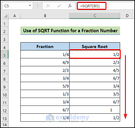
3. Apply the SQRT Function in Excel for a Fraction Number

Now, we will demonstrate how to apply the SQRT function to a fraction number in Excel. Follow the following steps.

• Firstly, to calculate the square root value for a fraction number, we have to type the following formula.

• Then, press Enter.
• Then, drag the Fill Handle icon to fill the other cells with the formulas.
• Therefore, you will get the following square root value for a fractional number.

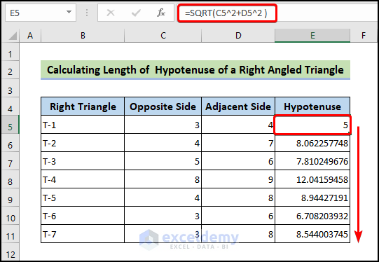
4. Calculating the Length of the Hypotenuse of a Right-Angled Triangle

According to the Pythagorean theorem, the square of a right-angled triangle’s hypotenuse is equal to the sum of the squares of its other two sides. The length of the hypotenuse can be determined using the SQRT function.

• Firstly, to calculate the length of the hypotenuse, we have to type the following formula.

• Then, press Enter.
• Then, drag the Fill Handle icon to fill the other cells with the formulas.
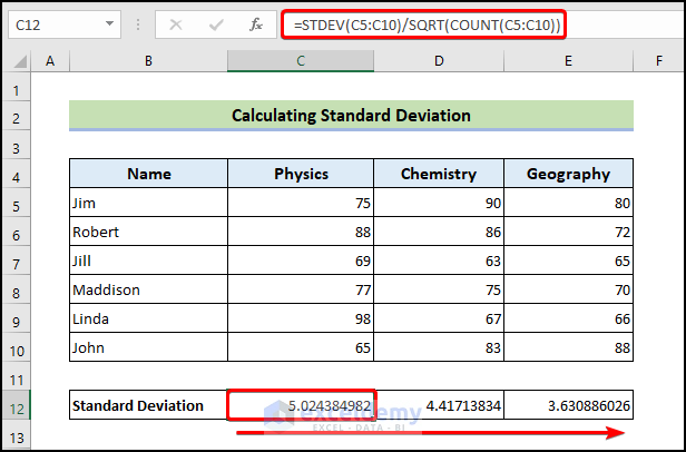
• Therefore, you will get the following length of the hypotenuse of a right-angled triangle.

5. Calculating Standard Deviation in Excel

We will show you how to compute the standard deviation in Excel using the SQRT function in the following example. The standard deviation is a measure of how variable your dataset is on average. It displays the average deviation from the mean of each statistic.

We will now use the following data set, which includes some names and grades in physics, chemistry, and geography.

• To begin, enter the following formula to calculate the standard deviation.

• Then, press Enter.
• Then, drag the Fill Handle icon to the right to fill the other cells with the formulas.
• Therefore, you will get the following standard deviation.

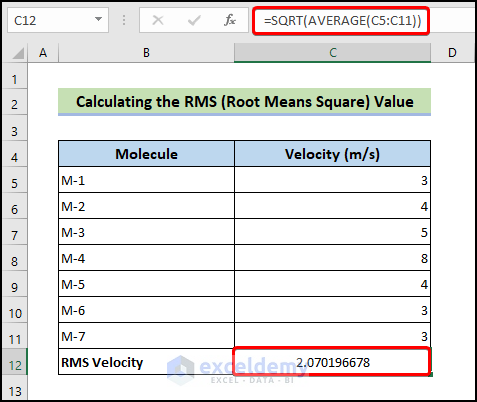
6. Calculating the RMS (Root Means Square) Value in Excel

In this example, we will demonstrate how to calculate the RMS value in Excel. The RMS (Root Mean Square) value, also known as the effective value or quadratic mean, is a mathematical measure that represents the magnitude of a varying quantity.

We will use the following dataset, which includes molecule number and velocity. Let’s walk through the following steps to determine the RMS velocity of the molecule.

• In order to calculate the RMS value, first enter the formula below.

Here, the AVERAGE function returns the average of the selected cell numbers.

• Then, press Enter.
• As a result, you will receive the RMS value as follows.

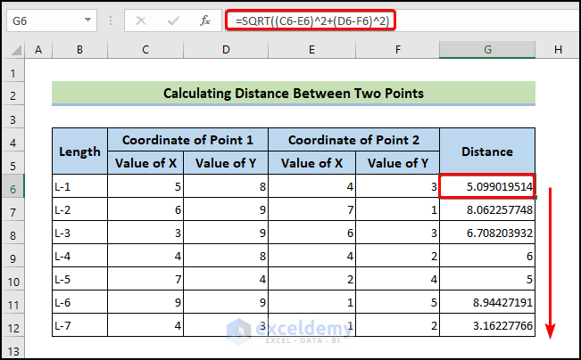
7. Calculating the Distance between Two Points in Excel

We can use the SQRT function to find the distance between two points in a two-dimensional plane. The following dataset, which contains the coordinate values for each point’s x and y, will be used. Let’s walk through the following steps to determine the distance between two points.

• Enter the following formula first in order to calculate the distance between two points.

• Then, press Enter.
• Then, drag the Fill Handle icon to fill the other cells with the formulas.
• As a result, you will receive the following distance between two points.

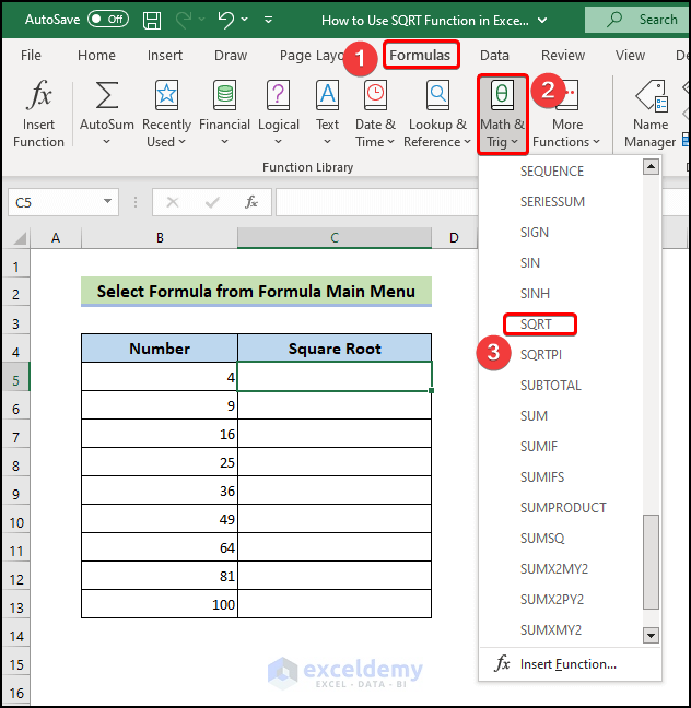
How to Apply SQRT Function Using the Formulas Main Menu of Excel

The SQRT function can also be accessed via the Formulas main menu.

• First, choose the final cell. Then go to the Formulas tab and select Math & Trig.
• Then, select SQRT from the drop-down option.

• Therefore, the Function Arguments dialog box will open.
• Enter the cell number in the Number section.
• Next, press Enter.

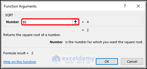
• Consequently, you will get the following square root value of cell B5.

• Then, drag the Fill Handle icon to fill the other cells with the formulas.
• As a result, you will receive the following square root value.

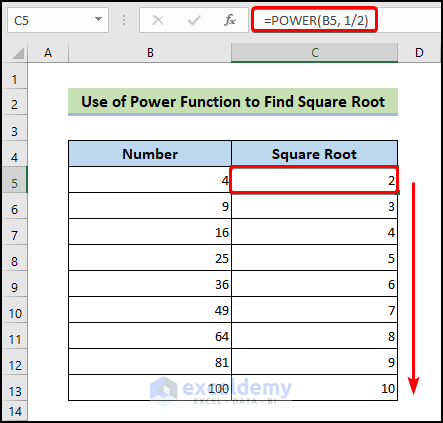
Find Square Root Without the SQRT Function (Using the Power Function)

The POWER function, unlike the SQRT function, can be used to calculate a number’s roots (such as square root or cube root) or powers (such as square or cube). The POWER function is essentially another way to do the square root, namely, raise a number to the power of 1/2.

• To begin, enter the following formula to find the square root.

• Then, press Enter.
• Then, drag the Fill Handle icon to the right to fill the other cells with the formulas.
• Therefore, you will get the following square root value.

Use VBA Code to Show the SQUARE Root of a Number in Excel

You can use VBA code to get the square root of a number. You have to follow the following steps.

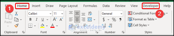
• VBA has its own separate window to work with. You have to insert the code in this window too. To open the VBA window, go to the Developer tab on your ribbon. Then select Visual Basic from the Code group.

• VBA modules hold the code in the Visual Basic Editor. It has a.bcf file extension. We can create or edit one easily through the VBA editor window. To insert a module for the code, go to the Insert tab on the VBA editor. Then click on Module from the drop-down.

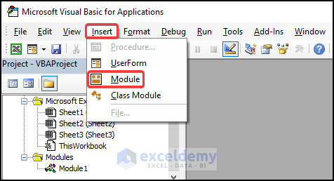
• As a result, a new module will be created.
• Now select the module if it isn’t already selected. Then write down the following code in it.

Sub SquareRoot()
Dim i As Integer
i = 5
Do While i < 12
Cells(i, 3) = Sqr(Cells(i, 2))
i = i + 1
Loop
End Sub

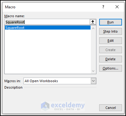
• Afterward, close the Visual Basic window. After that press Alt+F8.
• When the Macro dialogue box opens, select the following macro in the Macro name. Click on Run.

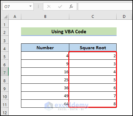
• Consequently, you will be able to calculate the square roots of the numbers.

How to Insert Square Root Symbol in Excel

In this additional method, we will add a square root symbol in our Excel sheet by using the UNICHAR function. The UNICHAR function displays a certain character in a cell if we pass the specific number assigned to that character as the argument of the function.

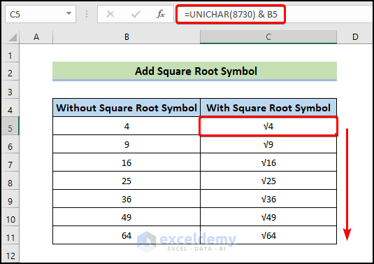
• Enter the following formula first in order to insert the square root symbol.

Here, we will pass the number 8730 as the argument of the UNICHAR function.

8730 is the number associated with the square root character. The ampersand sign will be used to concatenate square root symbol with cell B5.

• Then, press Enter.
• Then, drag the Fill Handle icon to fill the other cells with the formulas.
• As a result, you will receive the following square root symbol.

Common Mistakes When Using SQRT in Excel

The following are typical errors that people frequently make when use Excel’s SQRT function:

• If the input is a negative number:

Excel cannot determine the square root of a negative value, as was already established. The attempt will result in a #NUM! error. Make sure the input value is positive or zero to prevent this problem.

• If you forget to apply the parentheses:

Use parentheses to ensure the proper sequence of operations when combining the SQRT function with other functions.

Why Isn’t My SQRT Function Working?

If the SQRT formula isn’t functioning, think about the following potential problems:

• The value entered is negative.

As previously stated, Excel cannot calculate the square root of a negative value. A #NUM! error will be returned as a result of the attempt. To avoid this issue, make sure the input value is positive or zero.

• Use of parentheses incorrectly.

When using the SQRT function in conjunction with other functions, parentheses should be used to ensure the right order of operations.

• Typographical errors.

Verify your formula one more time for any errors, such as a misspelled function name or improper cell references.

How to Find Square Root Without SQRT Function in Excel

In this section, we will discuss 5 ways to find square roots in Excel. Firstly, we will use the exponent formula. Secondly, we will utilize the IF function. Thirdly, we will have the Nth root in Excel. In the next method, we will apply the SERIESSUM function to get the result. Then, we will opt for POWER QUERY to accomplish our task.

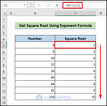
1. Get Square Root Using the Exponent Formula

When calculating manually, the radical symbol (√ ) is used to write the square root. Even though you can’t type the usual square root symbol in Excel, there is a way to find square root without using any functions. The caret character (＾), which is situated above the number 6 on most keyboards, is used for this.

• Firstly, to calculate the square root value using the exponent formula, we have to type the following formula.

• Then, press Enter.
• Then, drag the Fill Handle icon to fill the other cells with the formulas.
• Therefore, you will get the following square root value for the number.

2. Find Square Root Using the IF Function

In this following section, we will discuss finding square roots using the IF function. It’s a very important section while working with mixed data containing text values and numbers.

This square root expression can be utilized in larger formulations as well. For example, the IF statement below instructs Excel to generate a square root based on the following condition: If B5 includes a number, return a square root; if B5 is a text value or blank, return a blank cell.

• Firstly, to calculate the square root value using the IF function, we have to type the following formula.

The first argument, the ISNUMBER function checks whether the value in cell B5 is a number. If it evaluates to TRUE, the IF statement proceeds to the second argument

• Then, press Enter.
• Then, drag the Fill Handle icon to fill the other cells with the formulas.
• Therefore, you will get the following square root value.

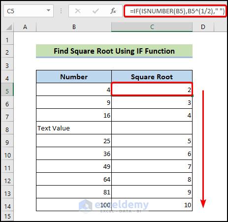
Therefore, you will see that it results in square root only for the numbers but blank values for the text values.

3. Calculate Nth Root in Excel

In case you need to calculate up to any root, a similar process to Method 1 can be followed to get up to the nth root of a particular number. Follow the following steps.

• Firstly, you have to calculate the square root value using the exponent formula in column C following Method 1.
• Next, we have to type the following formula in cell D5.

• Then, press Enter.
• Then, drag the Fill Handle icon to fill the other cells with the formulas.
• Therefore, you will get the following square root value.

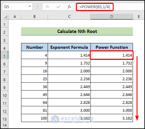
The exponential operator has the advantage of allowing you to calculate the square root, cube root, or nth root as well.

You can also use it to find the square, cube, or any power of the number.

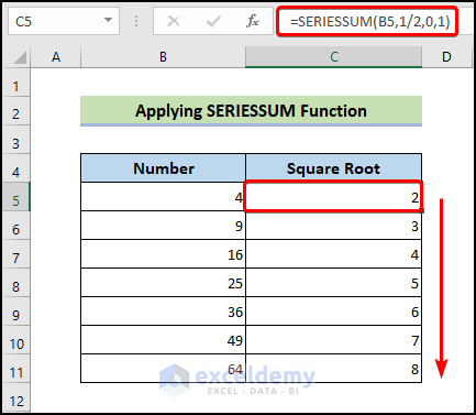
4. Calculate the Square Root with the SERIESSUM Function

The SERIESSUM function is used to calculate the sum of a power series. In this example, we will use the formula systematically to find the square root of different numbers.

• Firstly, to calculate the square root value using the SERIESSUM function, we have to type the following formula.

Here, the first value is the value at which we will evaluate the series. In this case, the value is cell B5.

The next argument is the starting power of the series. In our case, it is ½.

The subsequent argument is the progression in the series’ power increase.In this case, we do not want to increase our series power. Since we do have only one number. So, we will set the argument value to zero.

The final argument is the coefficients of the numbers in the series.In this instance, the only number we have is 4 and its coefficient is

• Then, press Enter.
• Then, drag the Fill Handle icon to fill the other cells with the formulas.
• Therefore, you will get the following square root value for the number.

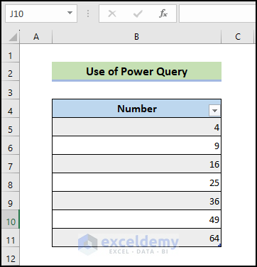
5. Calculate the Square Root with Power Query

In this method, we will use Power Query to add a column named “ Square Root” beside our existing dataset and then calculate the square root of the numbers.

📌 Steps:

• Firstly, we will convert our dataset into a table.
• To do this, select a data value from a dataset, go to the Insert tab, and from the Insert tab, select the Table option.

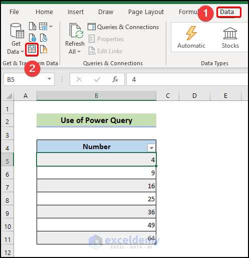
• After that, choose the Data tab from the ribbon.
• Then, select From Table/Range.

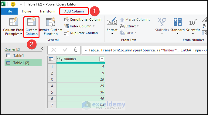
• In the Power Query window, first, go to the Add Column toolbar.
• From there select Custom Column.
• As a result, a window will pop up.

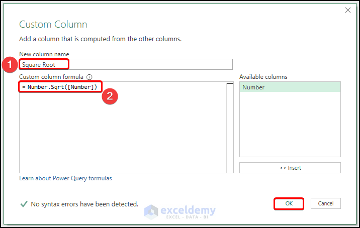
• In the Custom Column window, first, name the new column in the New column name box.
• In this instance, the name is Square Root.
• Then, in the Custom column formula write down the following formula

• Finally, click OK.

• After that, go to the Home tab of the Power Query window.
• From there, select the Close & Load tab.
• Finally, from the drop-down option select the Close & Load command.

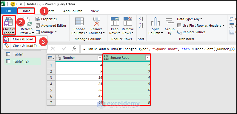
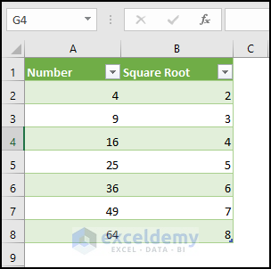
• Consequently, we will have the square roots of the numbers in a new window in a new column named “Square Root”.

FREQUENTLY ASKED QUESTIONS

1. Are there any limitations to using the SQRT function in Excel?

Yes, there are limitations to using the SQRT function in Excel. It can only find the square root of non-negative numbers, and it returns the positive square root of a given number. Additionally, the SQRT function has a limit to the number of decimal places it can return.

2. What other functions can I use in conjunction with the SQRT function in Excel?

You can use a variety of functions in conjunction with the SQRT function in Excel, depending on your specific needs. For example, you can use the SUM function to find the sum of a set of values before finding their square root, or the AVERAGE function to find the average of a set of values before finding their square root.

3. How do I format the output of the SQRT function in Excel?

You can format the output of the SQRT function in Excel by selecting the cell containing the function and then applying the desired formatting options, such as changing the number of decimal places, applying a currency format, or changing the font and cell color.

✍ Things to Remember

✎ Make sure that fractions (such as 1/2 or 1/3) are enclosed in brackets when applying the exponential operator. For Example, =4^(1/2) and =4^1/2  produce two different outcomes. This is because the exponential operator is calculated first, rather than division. The problem is solved by using brackets.

✎ A #NUM error will be returned if you use a negative number in the POWER function.

Download Practice Workbook

Download this practice workbook to exercise while you are reading this article. It contains all the datasets in different spreadsheets for a clear understanding. Try yourself while you go through the step-by-step process.

Conclusion

That’s the end of today’s session. I believe you will be able to use the SQRT function in Excel as of now. Through this article, you will learn 7 suitable examples of using the SQRT function with different number systems in Excel. The article is beneficial for those who want to simplify the process of getting square root values and save time in their data analysis work. Keep learning new methods and keep growing!

<< Go Back to Excel Functions | Learn Excel