Formatting a Chart in Excel – 8 Examples

Download Practice Workbook

Download the following workbook.

How to Insert a Chart from Data in Excel

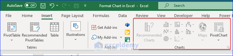
• Go to the Insert tab.
• Select a chart in Charts.

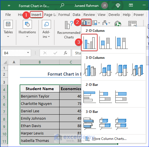
Here, Clustered Column in the 2-D Column:

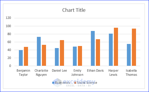
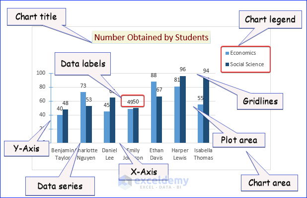
Chart Elements in Excel

Chart elements available in Excel:

• Axes
• Axis titles
• Chart titles
• Data labels
• Data table
• Error bars
• Gridlines
• Legend
• Trendline

Example 1 – Formatting X and Y Axis

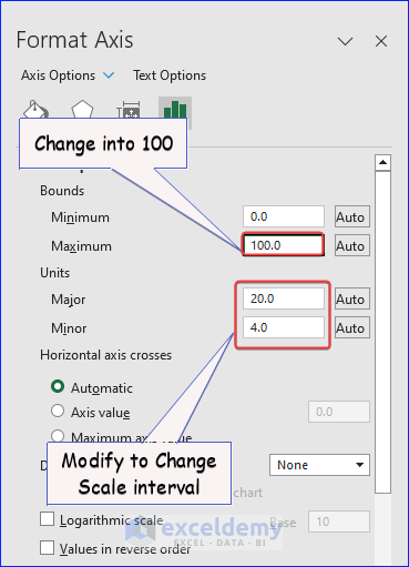
In the chart below the Y-axis scale starts at 0, and the scale expands up to 120 marks. To change it to 100 (the highest possible mark):

• Right-click the Y-axis and then select Format Axis.

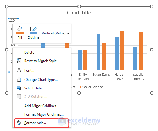
• In the Format Axis pane, change the value.

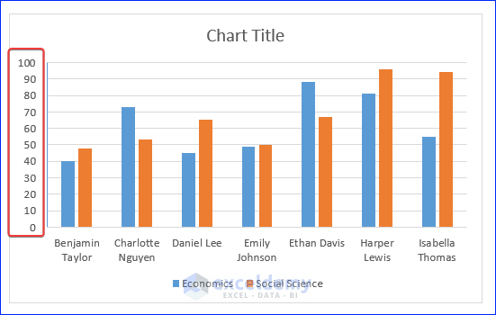
The highest value on the Y-Axis is 100.

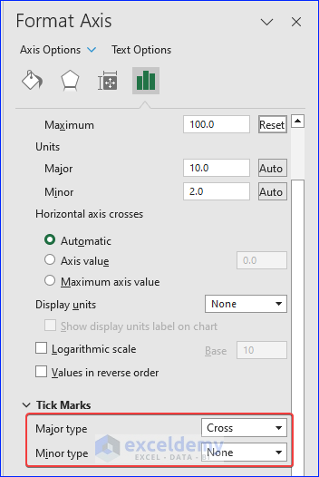
• Format the Y-Axis by adding Tick Marks next to the axis:

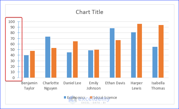
This is the output.

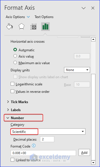
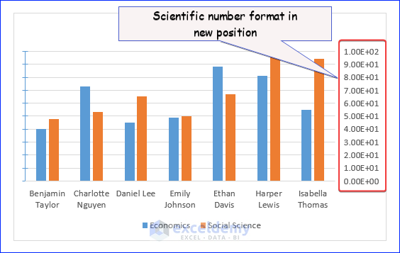
• Change the number format of the Y-Axis label to a Scientific number format.

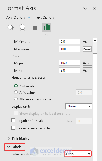
• Change the Label Position. Select High.

This is the output.

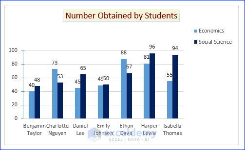
Example 2 – Formatting the Chart Title

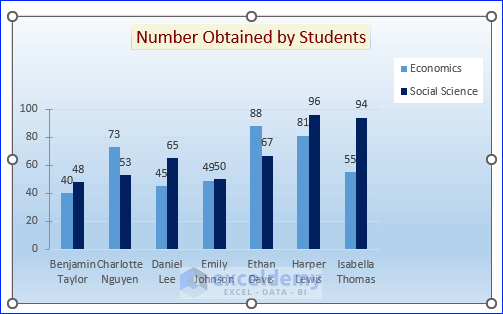
• Double-click the title and enter a new title. Here, “Number Obtained by Students”.
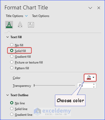
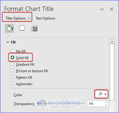
• Change the color of the text. In Text Fill, choose Solid Fill and choose a color.

• Change the Fill of the chart to Solid Fill and select a color.

This is the output.

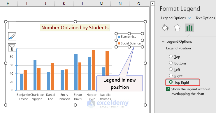
Example 3 – Format the Chart Legend 

• Click the chart legend to display Format Legend
• In Legend Options, click Top Right.

This is the output.

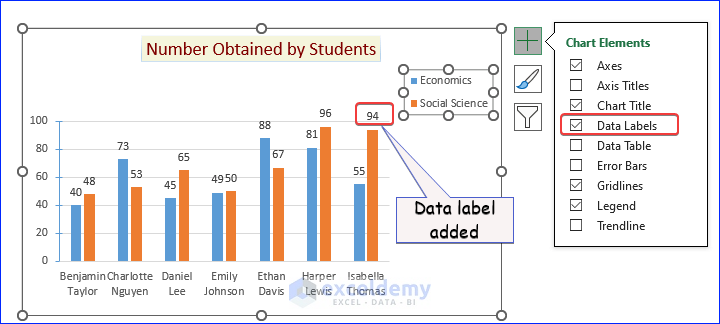
Example 4 – Format Data Labels 

Add data labels:

• Click  “+” 
• Check  Data Labels.

This is the output.

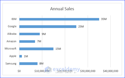
If you have large numeric values, the data label may be too large:

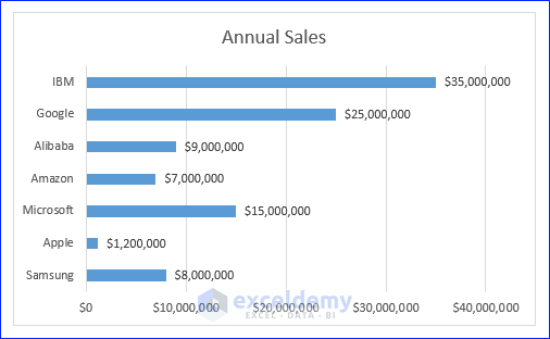
• Open Format Data Labels
• Click Number.
• In Category, select Custom.
• Enter the following format in the Format Code

This is the output.

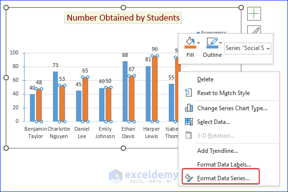
Example 5 – Formatting Data Series

• Click any column.
• Right-click and select Format Data Series.

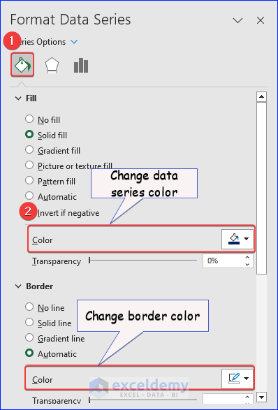
• In the Format Data Series pane, change the color to Navy-blue. You can also change the border color.

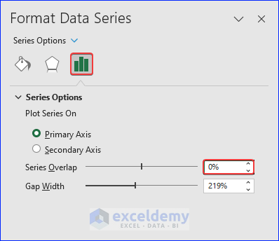
Change the distance between two adjacent columns in the chart:

• Click Series Options and change the Gap Width to “0”.

This is the output.

Read More: How to Change Chart Color Based on Value in Excel

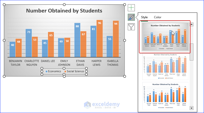
Example 6 – Change the Chart Style

• Click the chart, and you will find a “Paint brush icon” at the top-right corner.

• Click the icon to see the available charts. Choose one.

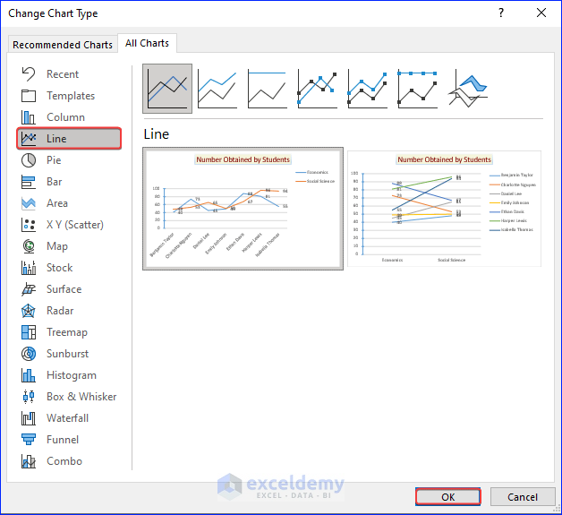
Example 7 – Change the Chart Type

• Right-click any column in the chart. Click Change Series Chart Type.

• In the Change Chart Type box, select a chart.

Example 8 – Formatting the Chart Area

The default chart area color is white. Change it:

• Change the color of the chart.

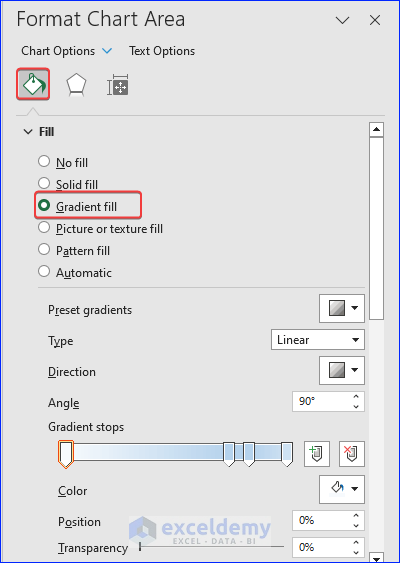
This is the output.

Read More: How to Make Excel Graphs Look Professional

Excel Charts Not Showing – Solution

• Go to File and then select Options.
• In the Excel Options, click Advanced and select For Object, Show:

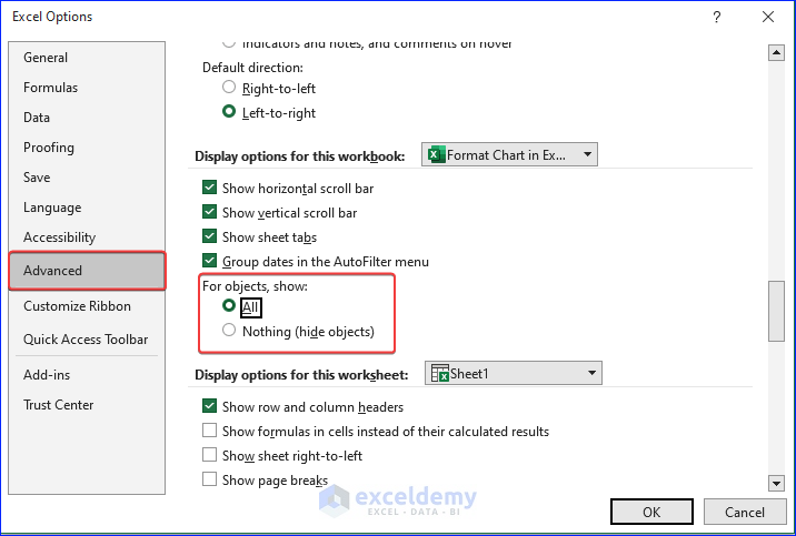
All types of charts are available in your worksheet.

Frequently Asked Questions

1. Is it possible to resize and move the chart to fit my worksheet better?

Yes, you can resize and move the chart by clicking it, and then dragging the handles.

2. Is it possible to format specific data points differently, like changing the color of a particular bar or data marker?

Right-click and use the Format Data Series option.

3. What is the difference between Chart Style and Chart Type?

Chart Type refers to the specific graphical representation of data whereas chart Style refers to the visual appearance and formatting applied to the chart elements.

Formatting Chart in Excel: Knowledge Hub

<< Go Back to Excel Charts | Learn Excel