If you want to add subscript(s) in an Excel graph, you have come to the right place. Here, we will walk you through 7 easy and effective methods to do the task smoothly.
Subscript in Excel: 7 Easy Methods to Add
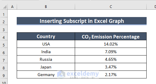
In the following dataset, you can see the Country and CO2 Emission Percentage columns. Next, using this dataset, we will go through 7 easy methods to add a subscript in an Excel graph. Here, we used Excel 365. You can use any available Excel version.
1. Using Copy and Paste Features to Insert Subscript in Excel Graph
In this method, we will use the Copy and Paste features to insert a subscript in an Excel graph. Here, we will add subscripts to the Chart Title using this method.
Let’s go through the following steps to do the task.
Step-1: Inserting Graph
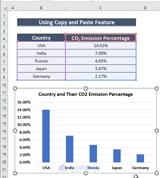
In this step, we will insert a Column chart.
- First of all, we will select the entire dataset by selecting cells B4:C9.
- After that, go to the Insert tab.
- Then, from the Insert Column or Bar Chart group >> select 2D Clustered Column Chart.

As a result, you can see the Column Chart.

- Then, we will edit the Chart Title.
Hence, you can see the chart with the chart title.
Here, you can easily notice that in the chart title CO2 does not have a subscript in it.
Furthermore, we will add a subscript to CO2.
Step-2: Adding Subscript in Graph
In this method, we will add a subscript to the Excel graph. To do so, we will copy the subscript from one cell, and then, we will paste it into the graph title.
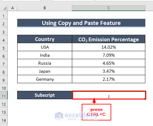
- In the beginning, we will type 2 in cell C11.

- Furthermore, to make the 2 a subscript, we will right-click on cell C11.
- Then, we will select Format Cells from the Context Menu.

At this point, a Format Cells dialog box will appear.
- Then, from the Font group >> we will mark Subscript >> click OK.

Therefore, you can see 2 in the subscript form.
- Moreover, we will copy this 2 by selecting cell C11 and pressing CTRL+C.
Afterward, we will go back to our graph and delete 2 from CO2.
- Then, we will paste the copied 2 after O by pressing CTRL+V.
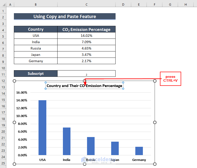
Hence, you can see, in the graph title, CO2 now has a subscript in it.
Therefore, we add a subscript in the Excel graph.

Read More: How to Rotate Text in an Excel Chart
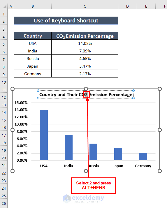
2. Use of Keyboard Shortcut to Add Subscript in Excel Graph
In this method, we will use the keyboard shortcut by pressing ALT+HFNB to add a subscript in the Excel graph.
Steps:
- First of all, we inserted the Column Chart and edited the Chart Title by following Step-1 of Method -1.
As a result, you can see the chart with the chart title.
Here, you can easily notice that in the chart title CO2 does not have a subscript in it.
Furthermore, we will insert a subscript to CO2.

- After that, to make the 2 a subscript in the Chart Title, we will select 2 and press ALT+HFNB.
Here, you must keep pressing the ALT key until you are finished pressing the other keys.
At this moment, you will see a Font dialog box will appear, and the Subscript is already marked.
- Then, we will click OK.

Hence, you can see, in the graph title, CO2 now has a subscript in it.
Therefore, we add a subscript in the Excel graph.

Read More: How to Change Text Direction in Excel Chart
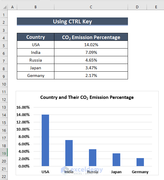
3. Using CTRL Key in Excel
Here, we will use the keyboard shortcut CTRL+1 to add subscripts in the Excel graph. Here, we will add a subscript in the Axis Title of a chart.
Steps:
- In the beginning, we inserted the Column Chart and edited the Chart Title by following Step-1 of Method -1.
As a result, you can see the chart with the chart title.
After that, to add Axis Title to the chart, we will click on Chart Elements.
- Then, we will mark Axis Titles.

- After that, we edited our horizontal and vertical Axis Titles.
Here, you can easily notice that the vertical Axis Title does not have a subscript in its CO2.

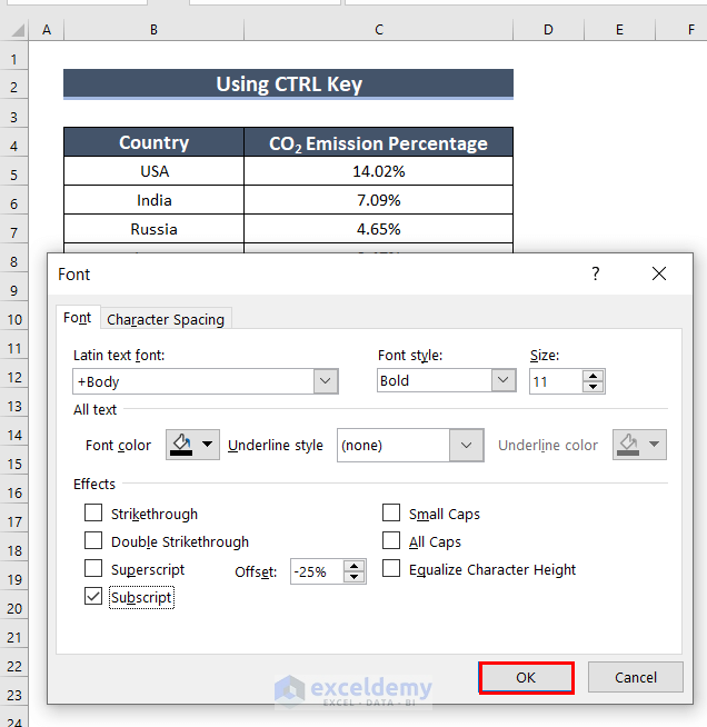
- Then, we will select 2 from the vertical Axis Title >> we will press CTRL+1.

At this point, a Font dialog box will appear.
You can see that the Subscript is already marked.
- Then, click OK.
As a result, you can see the subscript in the vertical Axis Title.

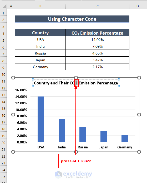
4. Inserting Character Code to Add Subscript in Excel Chart
In this method, we will use Character Code to add a subscript in the Excel graph.
Steps:
- In the beginning, we inserted the Column Chart and edited the Chart Title by following Step-1 of Method -1.
As a result, you can see the chart with the chart title.
Here, you can easily notice that in the chart title CO2 does not have a subscript in it.
Furthermore, we will insert a subscript to CO2.
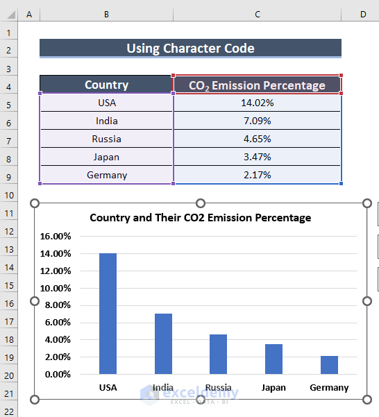
- After that, to make the 2 a subscript in the Chart Title, we will select 2 and press ALT+8322.
Note:
- One thing must be remembered we must press the code 8322 from the numbers side that is presented on the left side of the keyboard. The numbers that are presented in the upper position of the keyboard will not work.
- Or, you can type the numbers from the On-Screen Keyboard.
As a result, you can see in the graph title, CO2 now has a subscript in it.
Therefore, we add a subscript in the Excel graph.

Read More: How to Superscript Text in Excel Graph
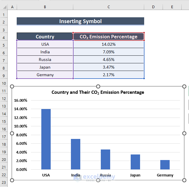
5. Inserting Symbol for Attaching Subscript in Excel Chart
Here, we will add a subscript by using a symbol in the data set. Using this method, we will add a subscript in the Legend of the graph.
Steps:
- In the beginning, we inserted the Column Chart and edited the Chart Title by following Step-1 of Method -1.
As a result, you can see the chart with the chart title.

As a result, you can see the Legend in the chart.
Here, although the column title in cell C4 has a subscript in it, the Legend does not have a subscript.
This is because the subscript of cell C4 is not presented in the Formula Bar.
Further, to add a subscript in cell C4 so that the Formula Bar also has a subscript, we will use Symbol.

- After that, we will delete the subscript 2 in cell C4 and we will put our mouse cursor after O.
- Then, we will go to the Insert tab >> from the Symbols group >> select Symbol.

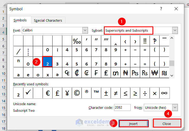
At this point, a Symbol dialog box will appear.
- Then, in the Subset box, we will select Superscript and Subscripts.
- Afterward, we will scroll down until we find 2.
- Here, since we need 2, we select 2.
- Moreover, we will click on Insert >> click Close.
As a result, cell C4 now shows a subscript in the Formula Bar.
Therefore, the Legend also has a subscript in it.

Read More: [Solved:] Vary Colors by Point Is Not Available in Excel
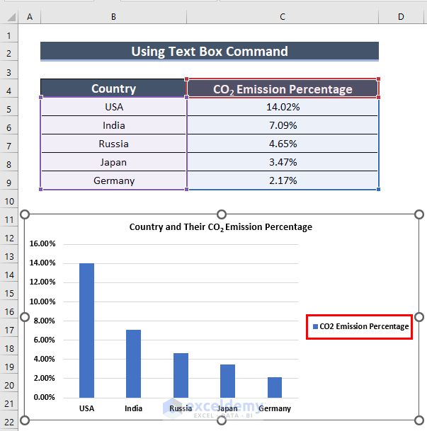
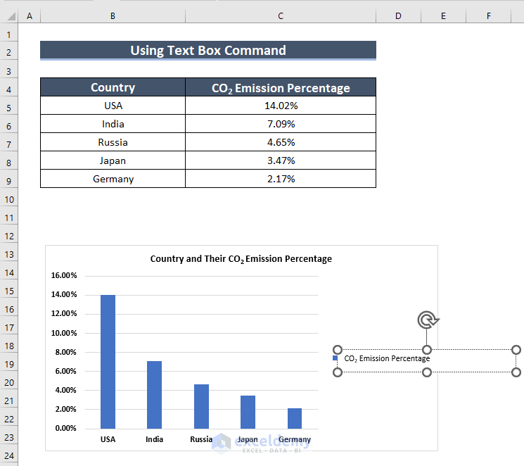
6. Using Text Box to Add Subscript in Excel Graph
In this method, we will use Text Box to add a subscript in Excel Graph. Using this method, we will add a subscript in the Legend of the graph.
Steps:
- In the beginning, we inserted the Column Chart and edited the Chart Title by following Step-1 of Method -1.
As a result, you can see the chart with the chart title.
- Furthermore, we add Legend to the chart by following the steps of Method-5.
Hence, you can see the chart with Legend.
Next, we will insert a Text Box where we will add a subscript, and we will place the Text Box in the position of the Legend.
- After that, we will go to the Insert tab >> from the Text group >> we will select the Text Box.

Then, you can see the Text Box.
- Afterward, we type CO2 Emission Percentage in the Text Box.
- Then, we add a subscript in the Text Box by following Method-2.

- Afterward, we drag the Text Box to the graph and place is over the Legend.
- Moreover, we click on the Text Box >> go to the Shape Format.
- Furthermore, from the Shape Outline group >> we will select No Outline.

Therefore, you can see the Legend has a subscript in it.

7. Use of Equation Feature in Excel
In this method, we will use the Equation feature from the Insert tab to add a subscript in the Excel graph. Here, using this method, we will insert a subscript in a chart Legend.
Steps:
- In the beginning, we inserted the Column Chart and edited the Chart Title by following Step-1 of Method -1.
As a result, you can see the chart with the chart title.
- Furthermore, we add Legend to the chart by following the steps of Method-5.
Hence, you can see the chart with Legend.
Next, we will insert an Equation where we will add a subscript, and we will place the Equation in the position of the Legend.
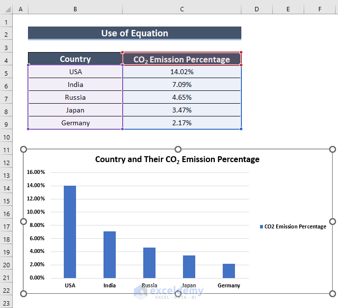
- In the beginning, we will go to the Insert tab >> from the Symbols group >> click on Equation.

At this point, an Equation box will appear.
- Moreover, from the Script group, we will select the equation that has a subscript form.

- Then, we will place the Equation form in the Equation box.

- Further, we will type the following text in the Equation box.
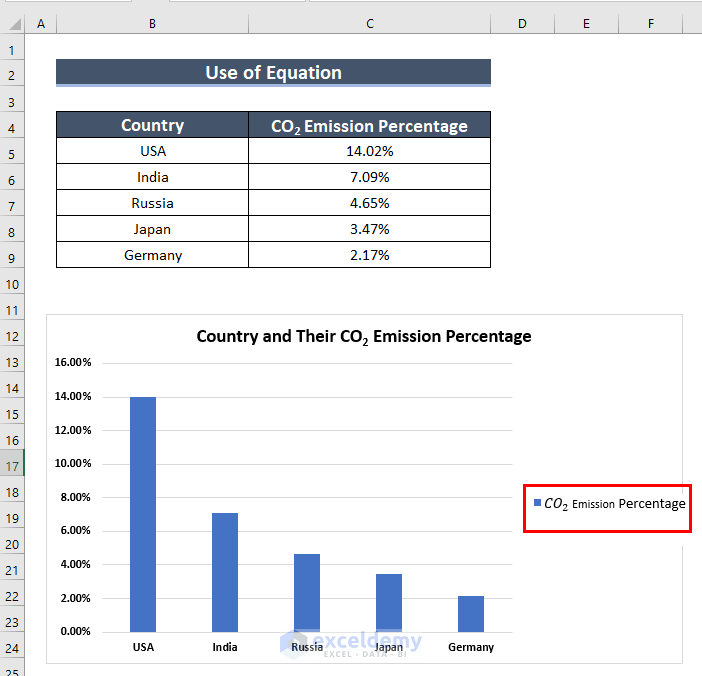
Then, we drag the Equation in the graph and place it on top of the Legend.
Hence, the Legend has a subscript in it.

- Then, we drag the Equation in the graph and place it on top of the Legend.
Hence, the Legend has a subscript in it.
How to Fix If Superscript Does Not Work in Excel
In the following data set, you can see we have Properties and Area (ft2) columns. Here, our superscript is not working, and therefore, we could not add superscript at ft2. Next, we will show you how you can solve the problem when the superscript is not working.

- First of all, we will click on the Customize Quick Access Toolbar.
- After that, we will select More Commands.

At this point, an Excel Options dialog box will appear.
- Furthermore, from the Quick Access Toolbar group, we will drag down until we find Superscript.
- Then, we will click on Add >> click OK.

Therefore, you can see a superscript.

- Then, we will select 2 from ft2 >> click on superscript.

As a result, you can see superscript in ft2.
Hence, the superscript is now working.

Practice Section
You can download the above Excel file to practice the explained method.

Download Practice Workbook
You can download the Excel file and practice while you are reading this article.
Conclusion
Here, we tried to show you 7 easy methods to add a subscript in an Excel graph. Thank you for reading this article, we hope this was helpful. If you have any queries or suggestions, please let us know in the comment section below.
Related Articles
- How to Show Coordinates in Excel Graph
- How to Make Excel Graphs Look Professional
- How to Change Chart Color Based on Value in Excel
<< Go Back to Formatting Chart in Excel | Excel Charts | Learn Excel
Get FREE Advanced Excel Exercises with Solutions!
