How to Superscript Text in Excel Graph (3 Quick Ways)

In terms of working with Microsoft Excel, you may occasionally need to use superscripts. Superscripts are small numbers or letters that appear slightly above the normal line of text. In this article, I am going to explain 3 quick ways on the matter of how to superscript text in Excel graph. I hope it will be helpful for you if you are looking for a way to superscript your Excel graph.

How to Superscript Text in Excel Graph: 3 Quick Ways

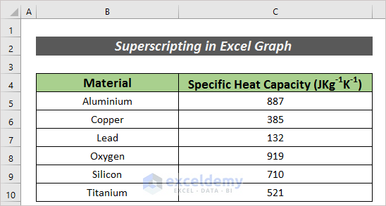
Superscript can be added in Excel graph quite easily. I am going to explain that in the later section. To simplify the explanation, I am going to use a dataset of specific heat capacity for different materials.

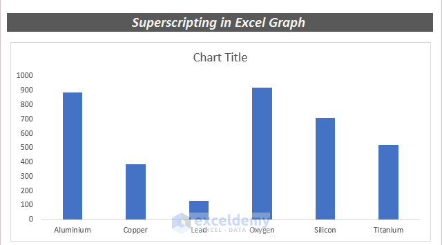
In order to make a graph with this dataset, go to the Insert tab. From the ribbon, pick Recommended Charts.

Thus, I have created an Excel graph with specific heat capacity.

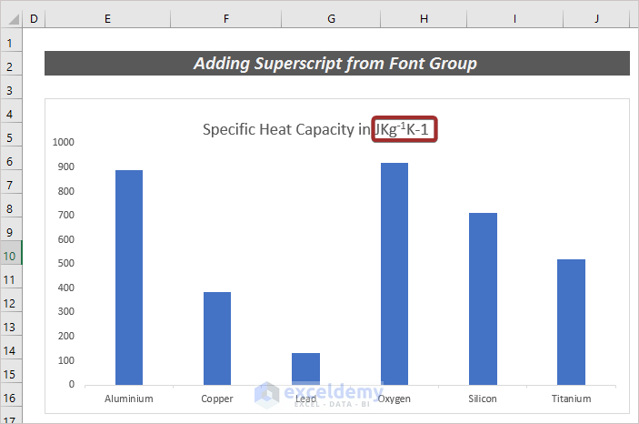
The unit of specific heat capacity is JKg^-1K^-1. So, we need to add superscript to show the unit in the graph.

1. Add Superscript from Font Group

As the simplest way, we can use the Font group under the Home tab to add superscript in graph. For details, see the following section.

Steps:

First of all, select the exact portion that you want to have as superscript.
Then, go to Home.
Next, click on the arrow in the Font group to extend the group.

A wizard named Font will pop up.

Check the Superscript box and click on OK.

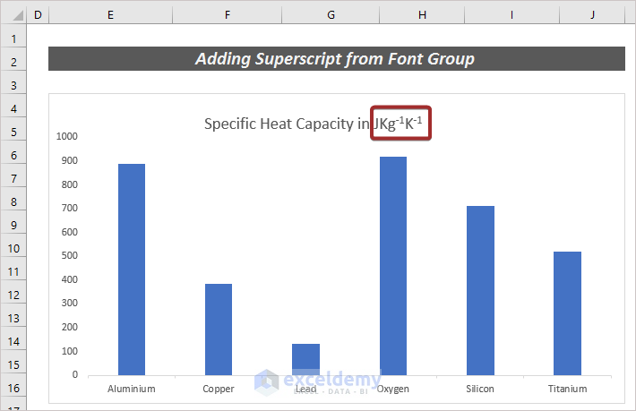
Thus, we will have the superscript in Excel graph.

Follow the similar procedure to superscript the rests.

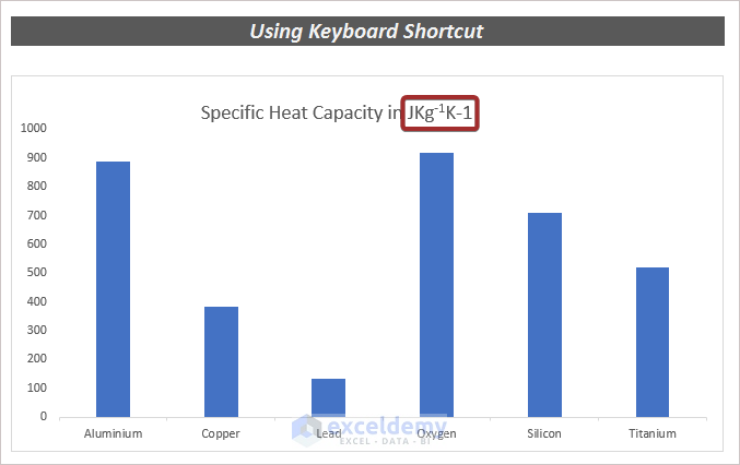
2. Use Keyboard Shortcut

In the previous method, we have used the Font wizard to superscript in Excel graph. We can to that in the shortest possible time using keyboard shortcut.

Steps:

Select the area that you want to have as superscript and press ALT + HFNP.

The Font wizard will appear along with the checked Superscript.

Click Ok to finish the process.

Finally, we have our desired output.

Similarly, you can superscript further if needed.

3. Apply Copy and Paste Method

Copy and Paste is probably the most useful function in Excel. We can use that here too.

Steps:

Write as a normal text in a cell that you want to have as superscript.
Next, select that cell and go to Home.
Click on the arrow in the Font group to extend the group.

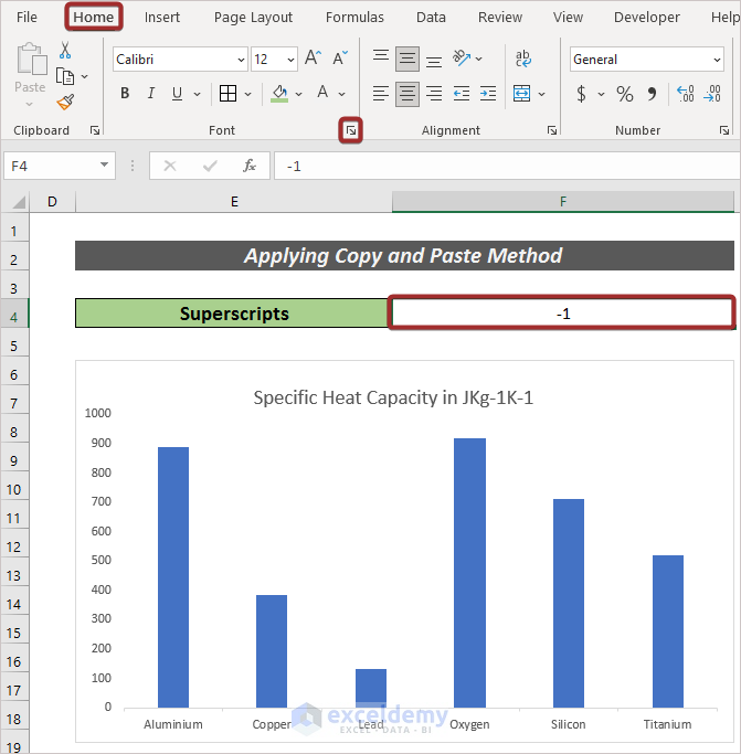
A wizard named Font will pop up.

Followingly, check the Superscript box and click on OK.

Thus, we will have a superscripted text in a cell.

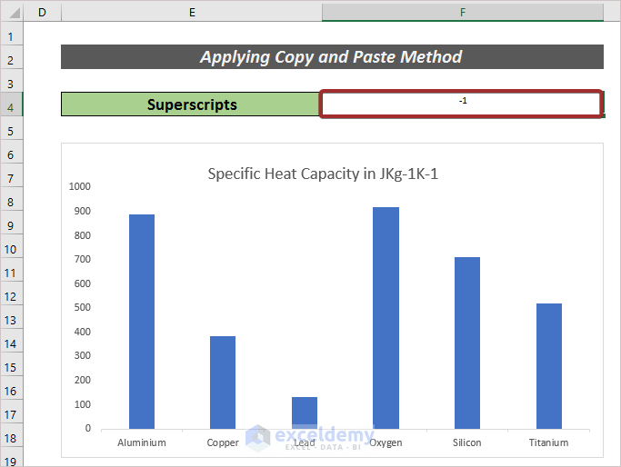
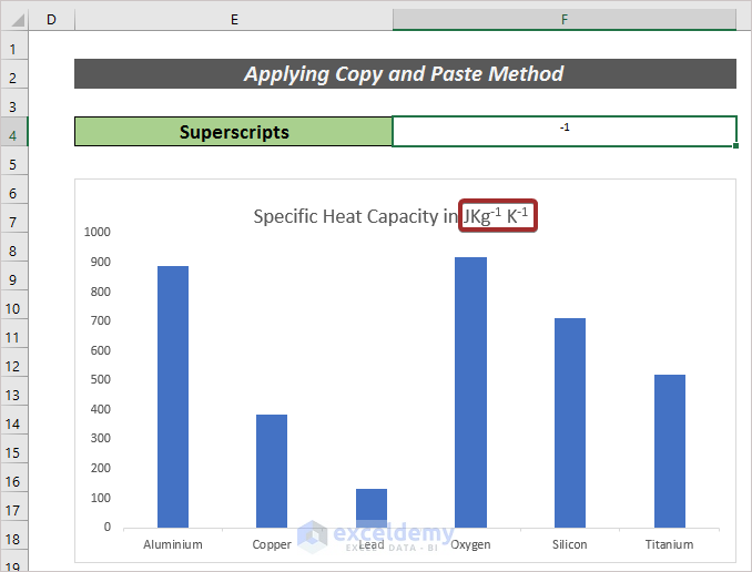
Now, Copy that cell and Paste it where necessary.

Download Practice Workbook

Superscript in Graph.xlsx

Conclusion

At the end of this article, I like to add that I have tried to explain 3 quick ways on the matter of how to superscript text in Excel graph. It will be a matter of great pleasure for me if this article could help any Excel user even a little. For any further queries, comment below. You can visit our site for more articles about using Excel.