Charts are very important tools to visualize and represent data attractively. While working with Excel charts, sometimes you need to Align the charts in Left, Right, or Center positions. Aligning a chart is a very easy process in Excel. In this article, I would like to show you how to left align a chart in Excel with 2 simple steps and necessary illustrations. I hope you will enjoy the process and can develop your Excel skills.
How to Left Align a Chart in Excel: Easy Steps
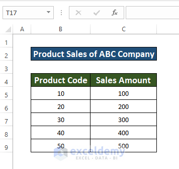
Let’s consider a dataset of Product Sales of ABC Company. The dataset has two columns B and C representing Product Code and Sales Amount. The dataset ranges from B4 to C9 cells. From here, I will explain how to left align a chart in Excel with the necessary steps and illustrations.
Step 1: Insert a Scattered Chart
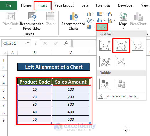
- First, Select the whole dataset.
- Then, Go to the Insert tab in your Toolbar.
- After that, Select the Scattered Chart
- Hence, Select the second option.
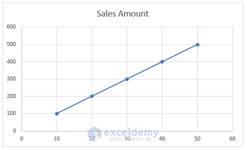
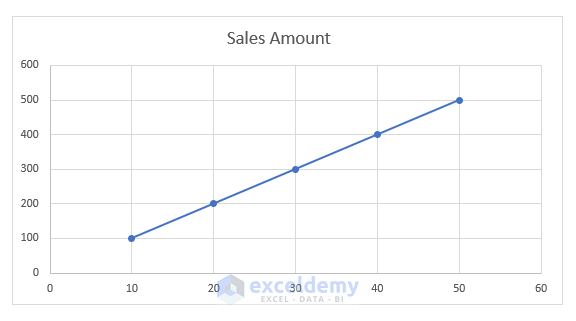
- Consequently, you will get the chart just like the picture given below.
Step 2: Align Chart on the Left Side
- Select the chart first.
- After that, you will find 8 points around the chart.
- Select any of the three indicated points.
- Then, Drag any of these three points.
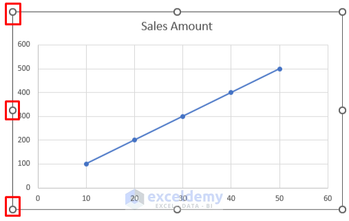
- As a result, you will find the newly aligned chart.
- You can also align two charts on the left side. First, apart from the scattered chart, Select the whole data table to insert a pie chart.
- After that, Go to the Insert tab in your Toolbar.
- Then, Select the Pie Chart.
- Hence, Select the 3-D Pie.
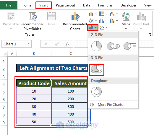
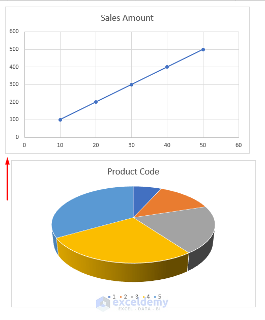
- As a consequence, You will find the pie chart like the picture given below.
- You will see that the pie chart is slightly displaced from the scattered chart on the right side.
- To solve this problem, first, Select a chart.
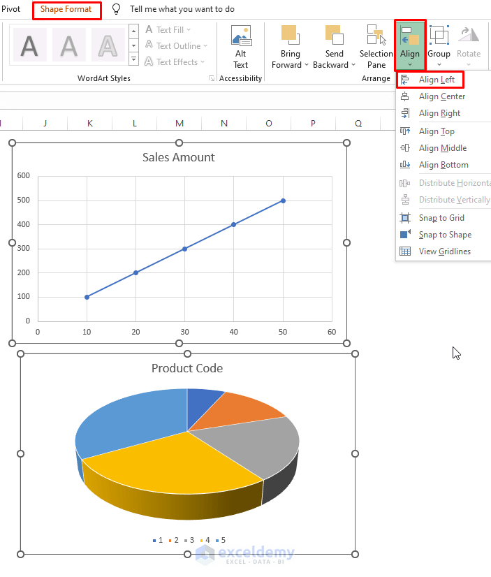
- After that, Select another chart by pressing the Shift.
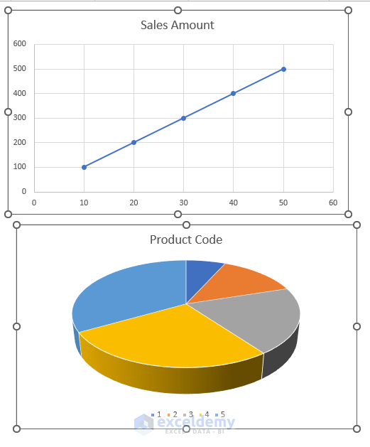
- After that, Go to the Shape Format option in your Toolbar.
- Moreover, Select the Align.
- Then, Press the Align Left.
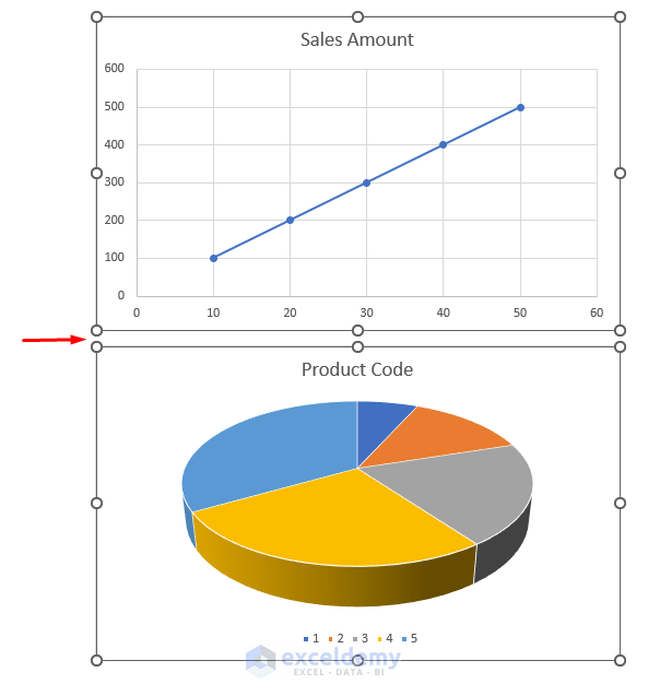
- As a result, you will find both of the charts are perfectly aligned on the left side.
Read More: How to Center a Chart in Excel
Things to Remember
- In step 1, we dragged the chart manually. If we want to put the chart’s corner on a cell’s corner, we need to drag and press the Alt key simultaneously.
Download Practice Workbook
Download the practice workbook to practice yourself.
Conclusion
In this article, I have tried to explain how to left align a chart in Excel. I hope you have learned something new from this article. Now, extend your skill by following the steps of these methods. I hope you have enjoyed the whole tutorial. If you have any kind of queries feel free to ask me in the comment section. Don’t forget to give us your feedback.
Related Articles
- How to Add a Vertical Dotted Line in Excel Graph
- How to Add Vertical Line in Excel Graph
- How to Add Border to a Chart in Excel
- How to Add Arrow in Excel Graph
- How to Add Asterisk in Excel Graph
- How to Remove Chart Border in Excel
<< Go Back to Formatting Chart in Excel | Excel Charts | Learn Excel
Get FREE Advanced Excel Exercises with Solutions!
