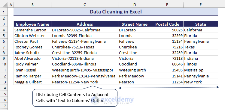
In this free Excel tutorial, we will explain the definition, importance, and several simple ways of data cleaning in Excel. We’ll use a dataset with employee info in the ‘Employee Name’ and ‘Address’ columns. The values in the ‘Address’ column are a compilation of street names, postal codes, and state names. As part of data cleaning in Excel, we have distributed cell contents to adjacent cells with the Text to Columns option.
We will also discuss the importance and challenges regarding data cleaning in Excel.
⏷What Is Data Cleaning in Excel?
⏷Importance of Data Cleaning
⏷Common Issues with Data That Need Data Cleaning
⏷Basics of Data Cleaning in Excel
⏷How to Clean Data in Excel?
⏵1. Checking the Spellings
⏵2. Highlighting the Duplicates
⏵3. Removing the Duplicates
⏵4. Replacing Text
⏵5. Changing Text Case
⏵6. Removing Spaces
⏵7. Removing Non-Printable Characters
⏵8. Fixing Numbers
⏵9. Fixing Times
⏵10. Fixing Dates
⏵11. Merging Columns
⏵12. Distributing Cell Contents to Adjacent Columns
⏵13. Switching Rows and Columns
⏵14. Reconciling Table Data
⏵15. Deleting All Formatting
⏵16. Highlighting Errors
⏵17. Sorting Data
⏵18. Removing Rows with Blank Cells
⏵19. Adjusting Rows and Columns
⏵20. Filling Blank Cells
⏵21. Formatting Data as Table
⏵22. Cleaning Data with Power Query
⏵23. Cleaning and Filtering Data with Pivot Table
⏵24. Changing Number Format into Percentage
⏵25. Finding Maximum and Minimum Values
⏵26. Filtering Data with “If Text Contains…” Feature
⏵27. Checking Data Types
⏵28. Adding Text at the Beginning
⏵29. Adding Text at the End
⏵30. Inserting Comma Before Nth Character from Right
⏵31. Removing Text Starting from a Particular Character
⏵32. Hiding Duplicate Rows
⏵33. Using Add-ins
⏷Challenges of Data Cleaning
What Is Data Cleaning in Excel?
Data Cleaning in Excel is a combination of processes that includes identifying, highlighting, and taking action against all kinds of errors to have organized data. There are many built-in Excel functions and features that are directly or indirectly used to ease the data-cleaning process in Excel.
Why Is It Important to Clean Data?
As we use data for many important decisions, it is a must to keep the data clean as far as possible. Some of the reasons are listed below:
- Accuracy: Ensures better accuracy while data is analyzed.
- Reliability: Instinctively enhances reliability.
- Efficiency: Reduces time spent on it as all the data are already sorted and ready to use.
- Better Decision-making: Less error-prone and helps to predict better decisions.
What Are the Common Issues with Data That Need Data Cleaning?
Data cleaning in Excel is a very vast section. Some of the most common issues with data that need cleaning include:
- Spelling mistakes
- Duplicate data
- Uncategorized text cases
- Unnecessary spaces, non-printable characters, and formats
- Unorganized formatting of numbers, times, and dates
- Missing text in a specific position, etc.
What Are the Basics of Data Cleaning in Excel?
The basics of data cleaning in Excel can be summed to these few steps:
- Import the raw data from an external data source.
- Keep a copy of the imported data in a separate workbook.
- Organize the data in table form with the right data in the right place.
- Make the data cleaning according to your needs.
How to Clean Data in Excel?
Method 1 – Spell-Checking
- Go to the Spelling option from the Review tab.
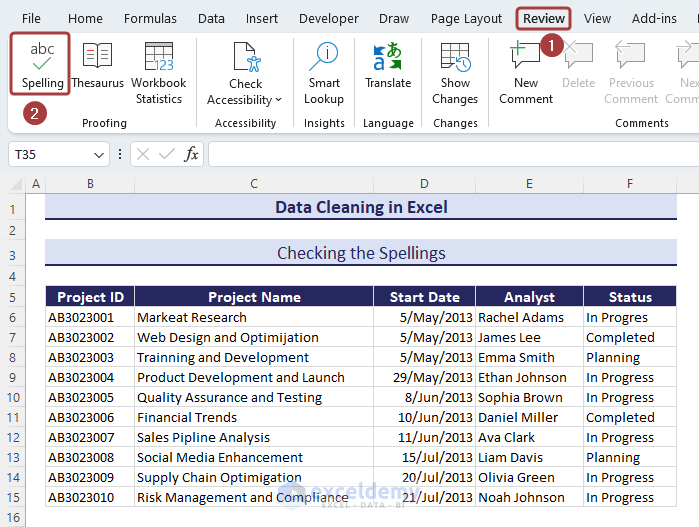
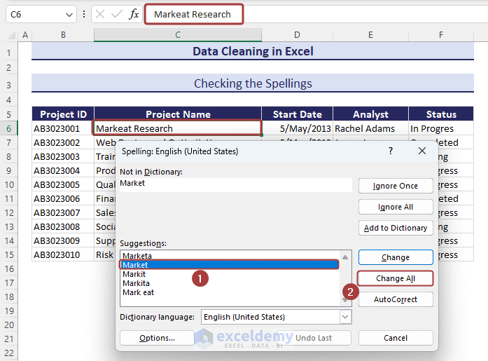
- A wizard named Spelling: English (United States) will appear with necessary suggestions of the misspelt words.
- Pick the correct spelling from the available spelling suggestions and click on Change All to make corrections in the entire worksheet.
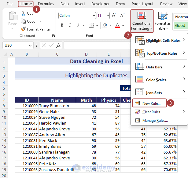
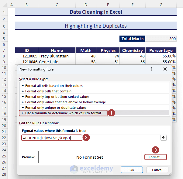
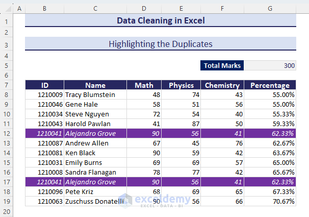
Method 2 – Highlighting Duplicates
- Go to Conditional Formatting from the Home tab.
- Select the New Rule… option.
- Pick the Use a formula to determine which cells to format option from the New Formatting Rule wizard.
- Insert the following formula in the Format values where this formula is true section:
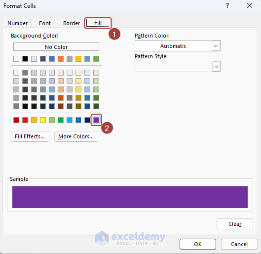
=COUNTIF($C$8:$C$19,$C8)>1- Click on the Format option to define the matched values format.
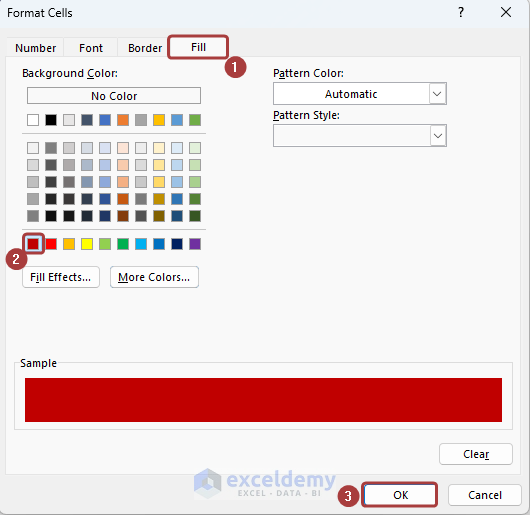
- Pick a background color from the Fill tab.
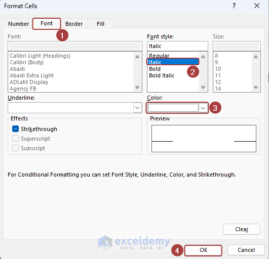
- You can customize the font style of the matched values. We have set the font color white and style italic for the matched cells.
- Click OK to finish the formatting.
- Click OK again to apply the conditional formatting.
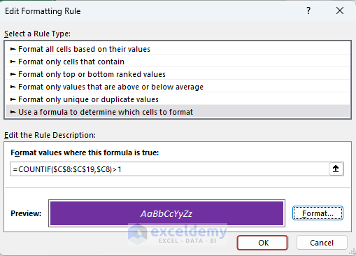
- We have the duplicate values highlighted according to the defined formatting.
Method 3 – Removing Duplicates
- Select the entire data and go to the Data tab.
- Click on Remove Duplicates.
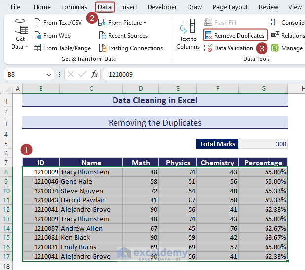
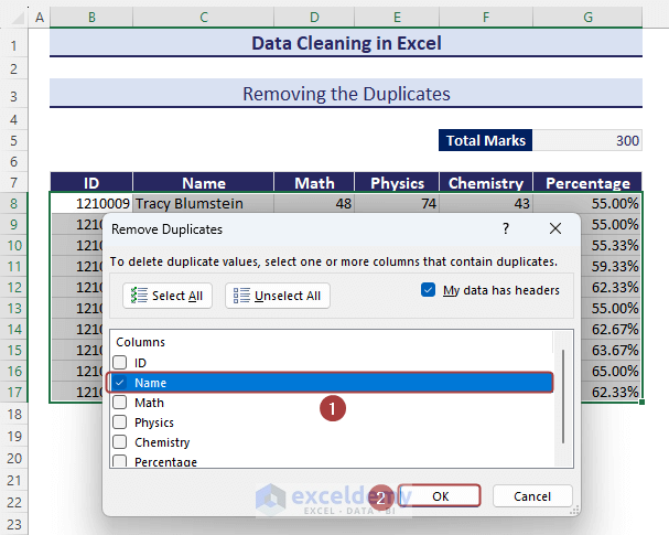
- Pick a column and click on OK to find the duplicates and delete the entire row.
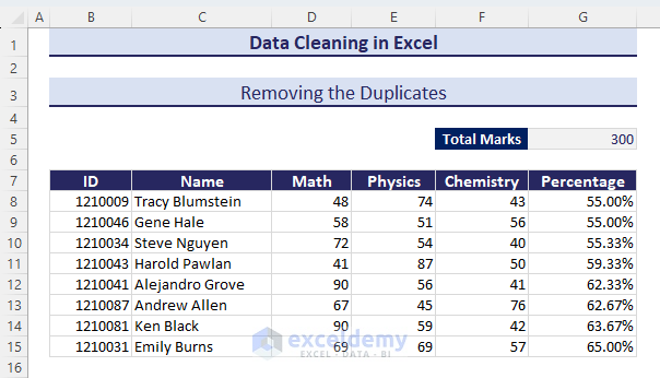
- We’ll get a dataset with no duplicates along the defined column.
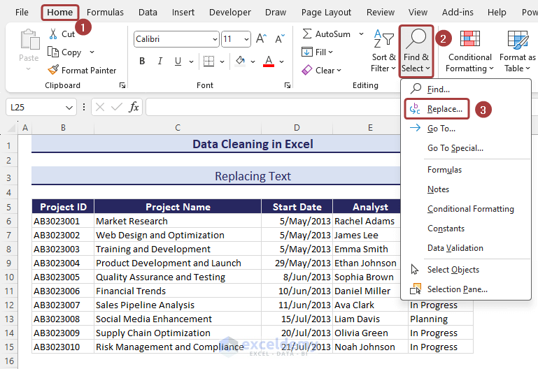
Method 4 – Replacing Text
- Go to the Find & Select command from the Home tab.
- Pick Replace… from the available options.
- Input the text to be replaced (i.e. In Progress) in the Find what section and the text that will be inserted (i.e. Completed) in the Replace with section.
- Click on Replace All.
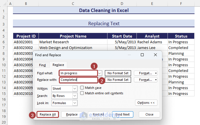
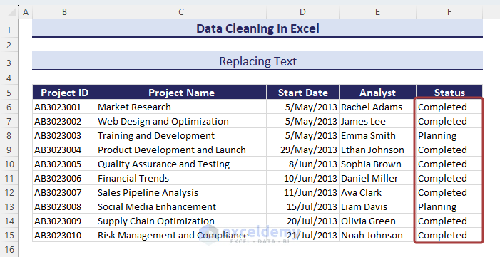
- Thus, we can simply replace texts.
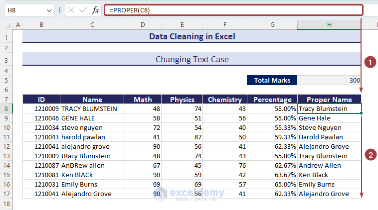
Method 5 – Changing Text Cases
- Apply the following formula with the PROPER function in cell H8 to have the name of cell C8 in the proper case:
=PROPER(C8)- Use the Fill Handle to autofill the formula.
Method 6 – Removing Spaces
- Apply the following formula with the TRIM, CLEAN, and SUBSTITUTE functions to remove spaces between texts as well as leading spaces at the beginning:
=TRIM(CLEAN((SUBSTITUTE(C6,CHAR(160)," "))))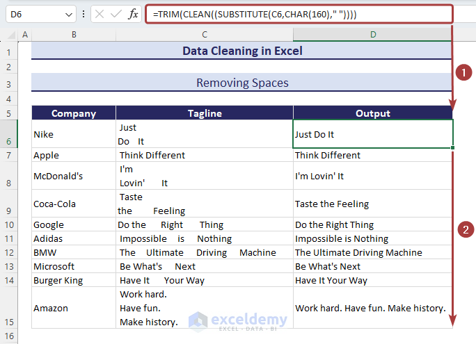
Method 7 – Removing Non-Printable Characters
Look at Column C, under the Name header, and you’ll find some unwanted characters before or between texts that are not printable.
- Apply the following formula with the CLEAN function to have the non-printable characters removed:
=CLEAN(C8)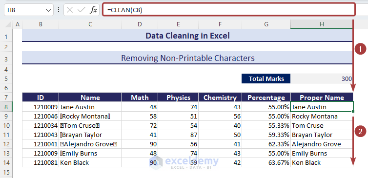
Method 8 – Fixing Numbers
- Use the following formula with the VALUE function to put the numbers in the number format.
=VALUE(F6)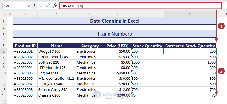
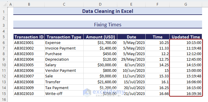
Method 9 – Fixing Times
Times in general format show a numerical value. We need to change the number format to have them in the time format.
- Apply the following formula into the result cells to convert them to hours:
=F6/24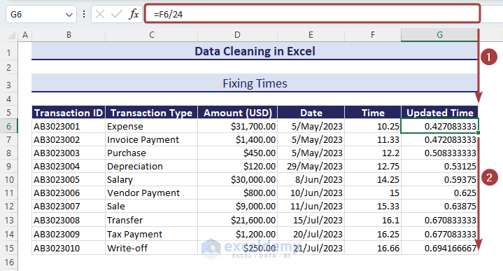
- Select all cells in general mode and select Time from the Number Format option.
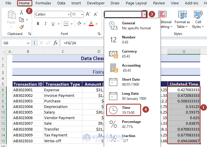
- We’ll get the time in a proper format.
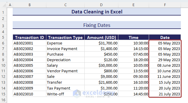
Method 10 – Fixing Dates
Excel stores dates as sequential serial numbers. If they are not assigned a Date format, they might appear as vague 5 or 6-digit numbers.
- Select the cells containing the dates represented as numbers.
- Choose Short Date or Long Date from Number Format to have the numerical values in proper date format.
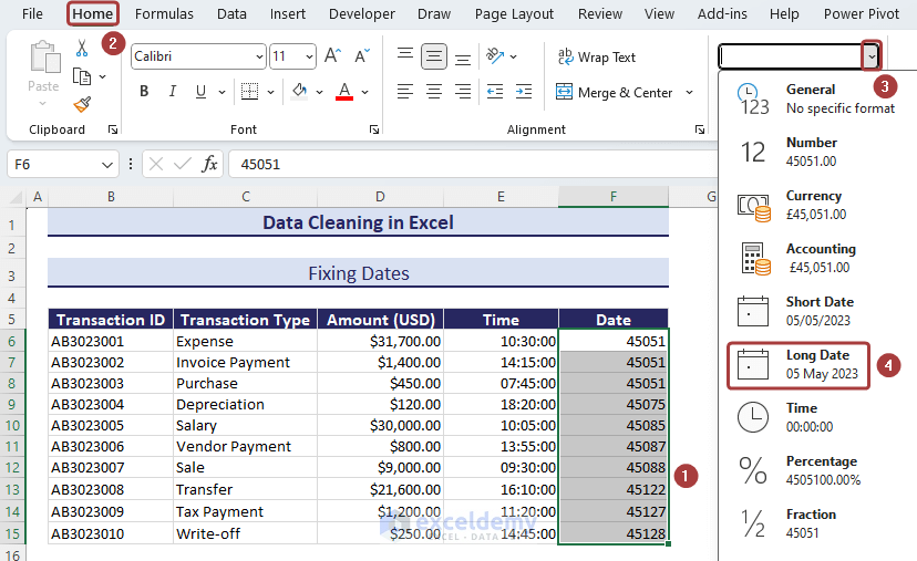
- This will fix most date issues.
Method 11 – Merging Columns
Under the Address header in column F, we’ll show the proper address format by merging the street name, postal code, and state name from the left 3 columns.
- Apply the following formula with the CONCATENATE function to merge the columns and separate the segments with dashes:
=CONCATENATE(C6,"-",D6,"-",E6)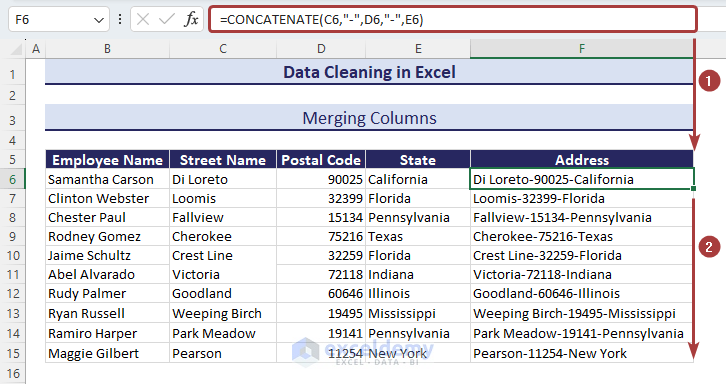
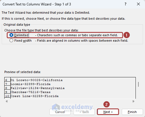
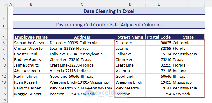
Method 12 – Distributing Cell Contents to Adjacent Columns
We have a dataset where the addresses are the combination of the street name, postal code number, and state name. Those are separated with a dash (–) between them.
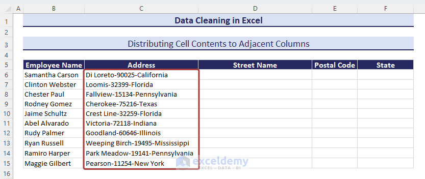
- Copy the entire column values to the Street Name column.
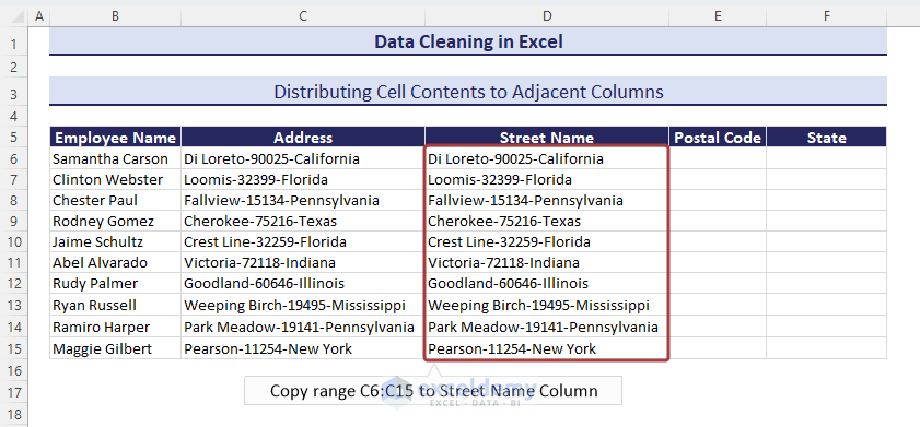
- Select all the values in the Street Name column and click on the Text to Columns option from the Data tab.
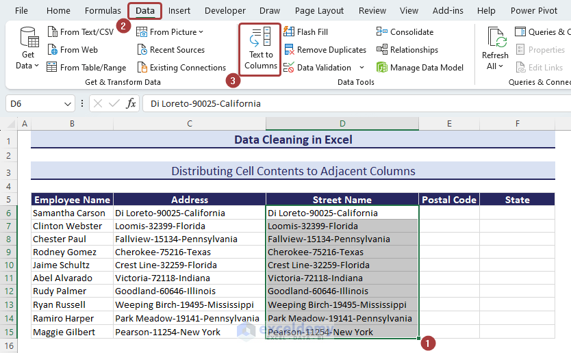
- From the Convert Text to Columns Wizard, choose the Delimited since the data is combined with the dash sign.
- Click on Next.
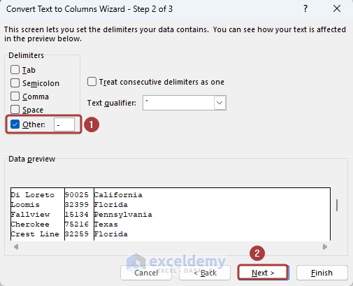
- Define the delimiter based on what the cell values are separated.
- Click on the Next button.
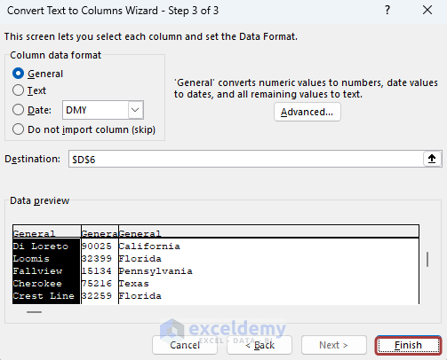
- Click on Finish to end the process.
- We have the distributed cell values in the adjacent cells.
Method 13 – Switching Rows and Columns
- Copy the entire range.
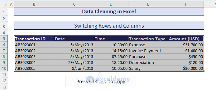
- Select a cell to paste the switched rows and columns.
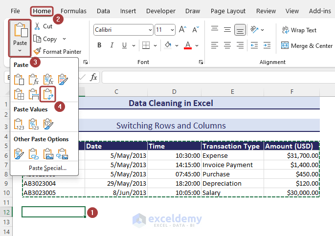
- Go to Paste from the Home tab.
- Pick the Transpose (T) option to make the switch.
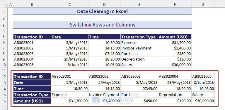
- We’ll get the switched rows and columns.
Method 14 – Reconciling Table Data
In the following dataset, we have two tables that represent sales amounts in June and July. We will reconcile them to know the status of whether the sales amount has changed or not.
- Apply the following formula to reconcile the data of two tables and have the status “Changed” or “Unchanged”:
=IF(F6=C6,"Unchanged","Changed")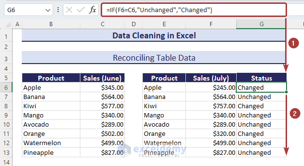
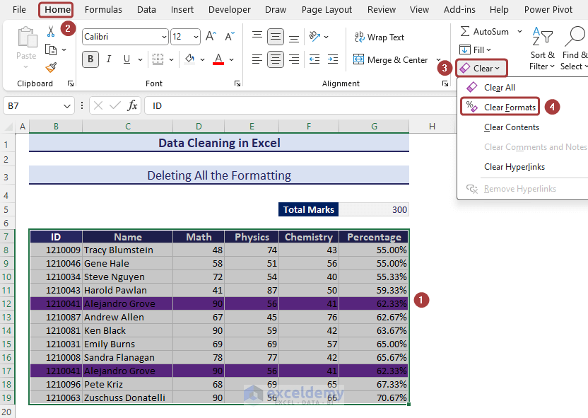
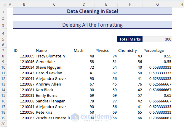
Method 15 – Clearing Formatting
- Select the entire data and go to Home.
- Click on Clear Formats from the Clear option to remove the formatting.
- We’ll have just raw data without any formatting.
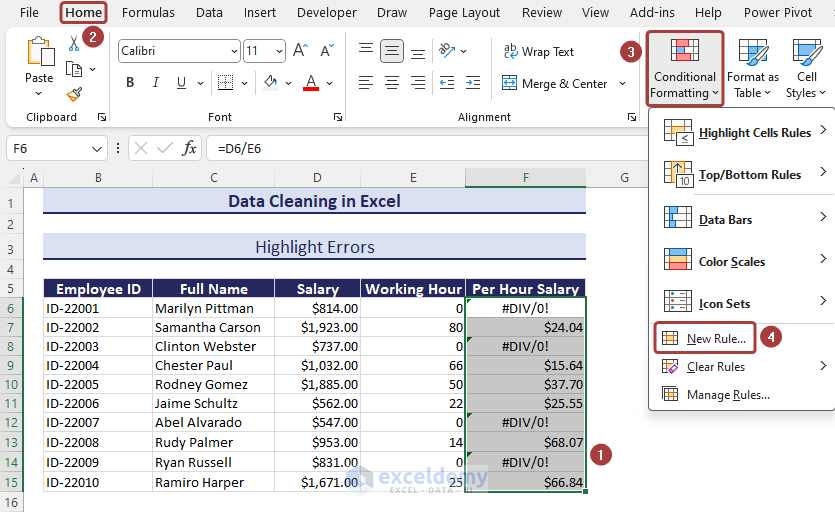
Method 16 – Highlighting Errors
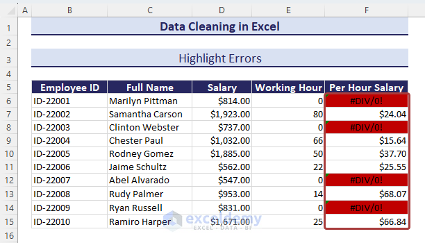
In the Per Hour Salary column F, some cells return errors instead of any proper values.
- Select the entire area where you want to highlight errors.
- Click on Conditional Formatting from the Home tab and select New Rule…
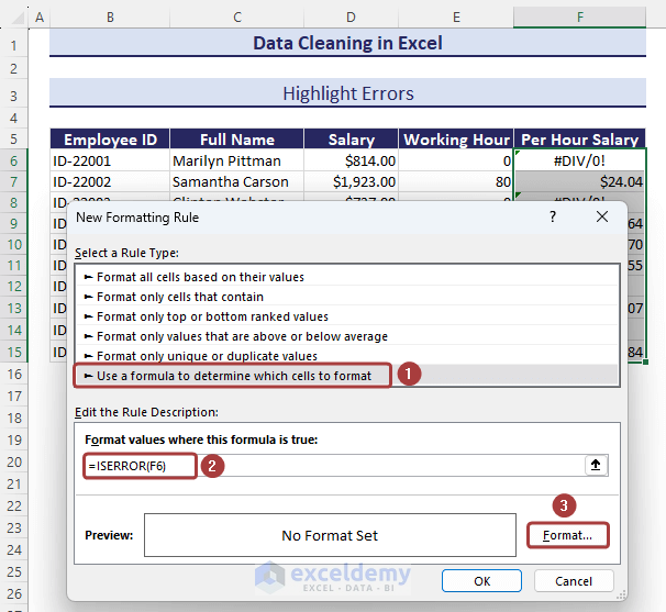
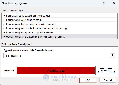
- Choose the Use a formula to determine which cells to format option from the New Formatting Rule wizard.
- Copy the following formula in the Format values where this formula is true section.
=ISERROR(F6)- Click on the Format option to define the matched values format.
- Pick a background color from the Fill tab and click on OK.
- Click OK again to apply the conditional formatting.
- The cells containing errors will be highlighted.
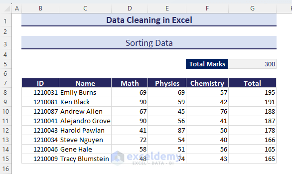
Method 17 – Sorting Data
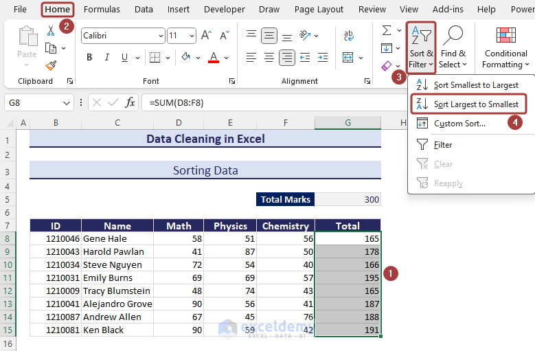
In the following dataset, we will sort data in descending order based on the total marks.
- Select the column you want to sort by.
- Go to the Home tab and click on Sort Largest to Smallest from Sort & Filter to sort in descending order.
- Choose the Expand the selection option and click on Sort.
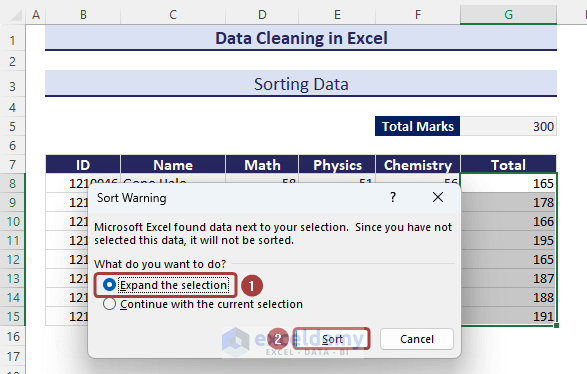
- We have the table sorted in descending order.
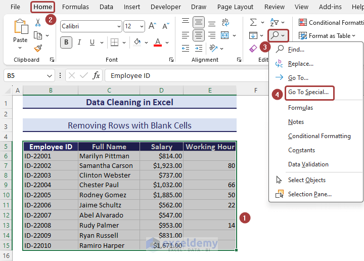
Method 18 – Removing Rows with Blank Cells
In the Working Hour column, we can see that some of the cells are empty. We will remove the entire rows for those cells.
- Select the entire dataset and go to Home.
- Pick the Go To Special… option from the Find & Select group.
- Select the Blank option and click on OK in the Go To Special wizard.
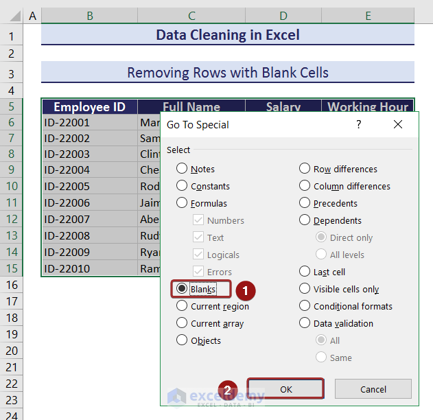
- All the blank cells are selected within the selected range.
- Go to the Home tab again.
- Click on the Delete Sheet Rows option from the Delete feature.
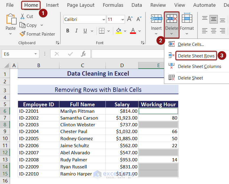
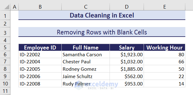
- We’ll get a clean dataset without rows with blank cells.
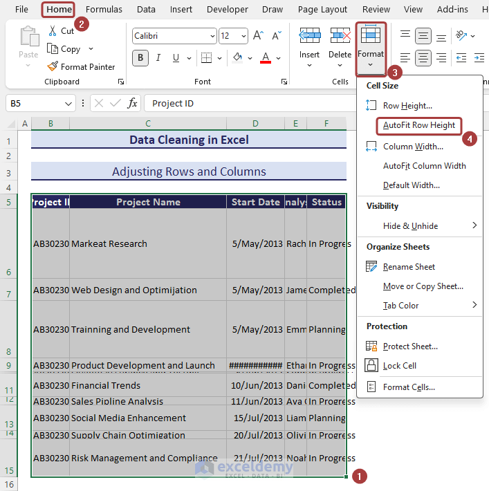
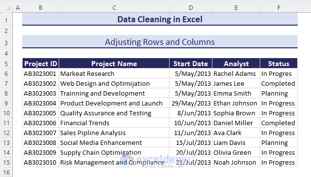
Method 19 – Adjusting Rows and Columns
In our dataset, the row heights and column widths are not identical in all cases.
- Select the entire dataset and go to Home.
- Go to the Format feature and pick the AutoFit Row Height option for row adjustment.
- Select the AutoFit Column Width option from the Format feature for column adjustment.
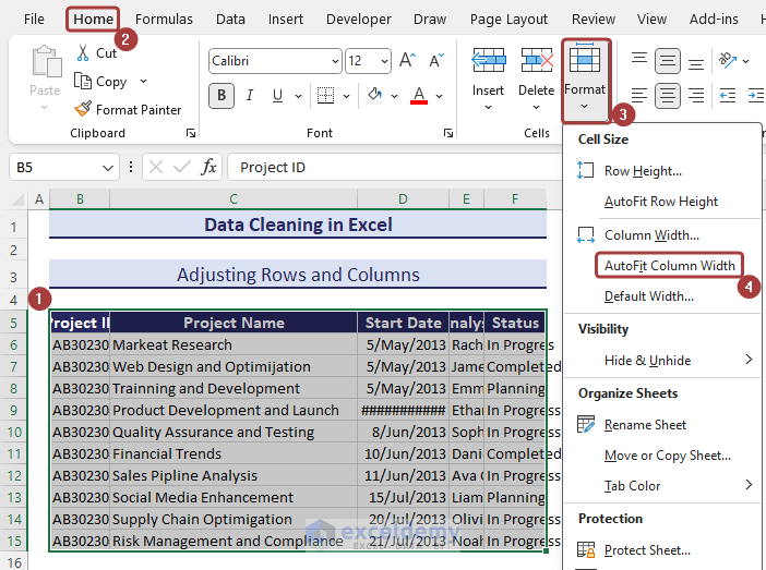
- We have a more organized dataset with adjusted rows and columns.
Method 20 – Filling Blank Cells
Blank cells make a dataset unfulfilled. We can insert zeros in those cells to have a better representation.
- Select the entire range.
- Go to the Home tab and select Find & Select from the ribbon.
- Pick Go To Select… from the available options.
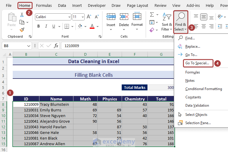
- Select Blanks and click on OK.
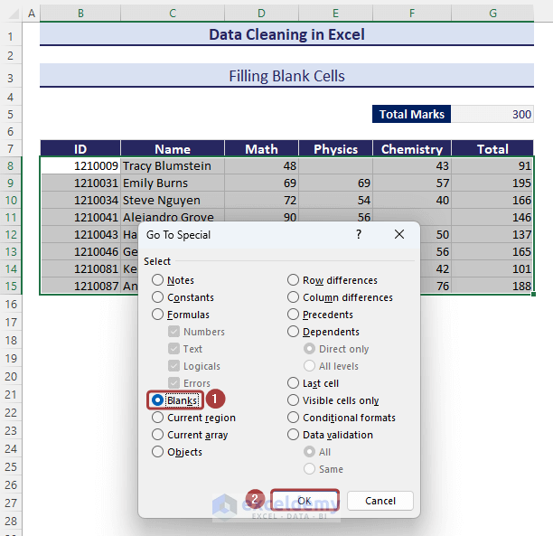
- The blank cells within the selected range will be selected.
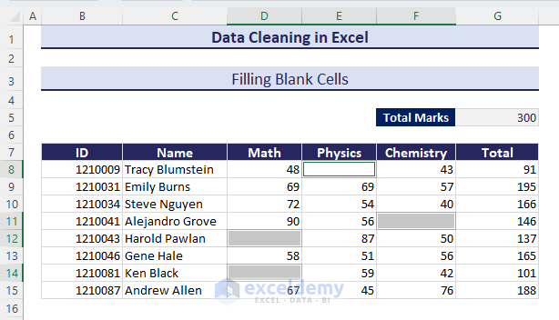
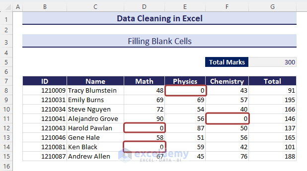
- Insert zero and press Ctrl + Enter.
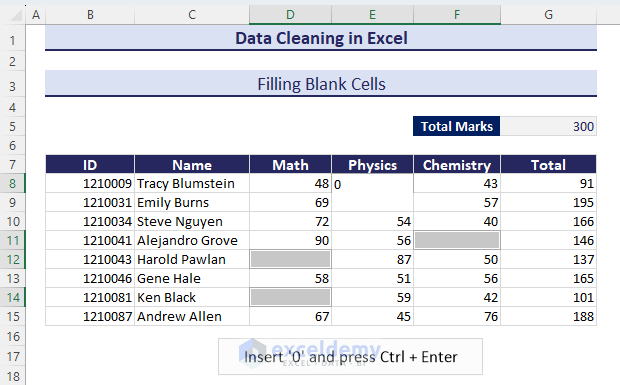
- We will have the blank cells filled with zeros.
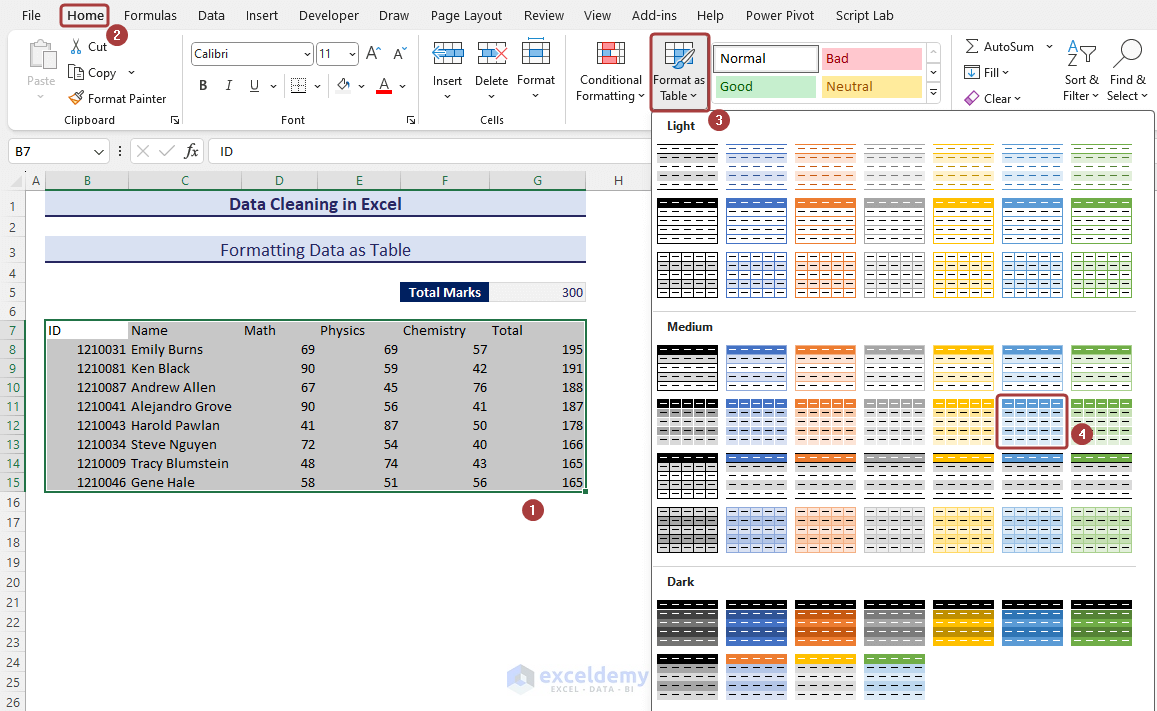
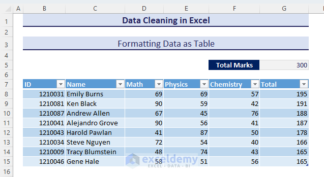
Method 21 – Formatting Data as a Table
- Select the entire range of data.
- Go to Home and select Format as Table from the ribbon.
- A dialog box named Create Table will appear to make the confirmation of your table range. You can change the table range that was previously defined by selection.
- Check the My table has headers box if you have headers.
- Click on OK to finish the process.
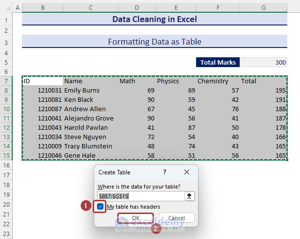
- We will have data presented as a table.
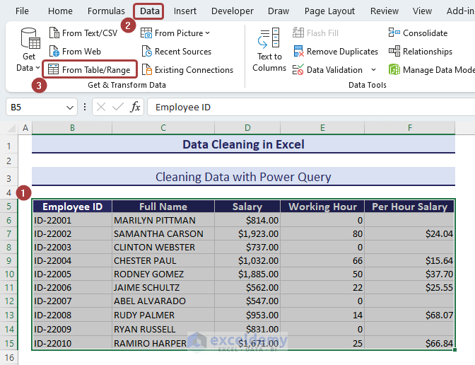
Method 22 – Cleaning Data with Power Query
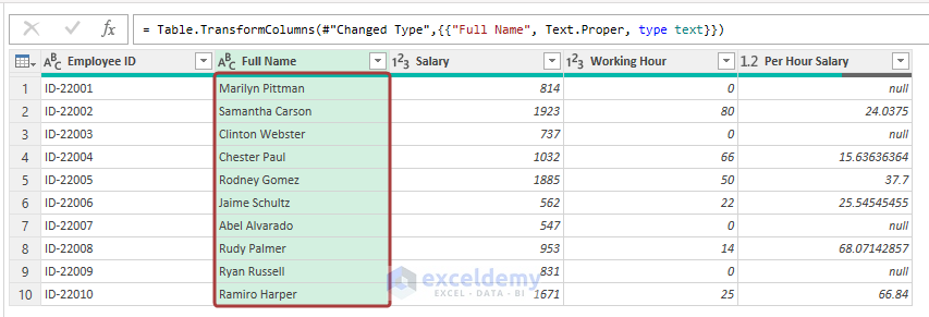
We have a dataset where names are written in capital letters. There are also some empty cells in the Per Hour Salary column. Let’s change the names into the proper case and delete the rows with empty cells.
- Define a range to apply the Power Query feature.
- Go to Home and select From Table/Range from the ribbon.
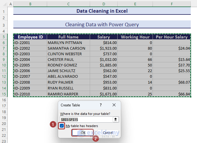
- Confirm the table range and check the My table has headers box if you have headers.
- Click on OK.
- The table will appear in the Power Query Editor.
- To change the case of the names into the proper format, select the Full Name column and go to the Transform tab.
- Pick the Capitalize Each Word option from Format.
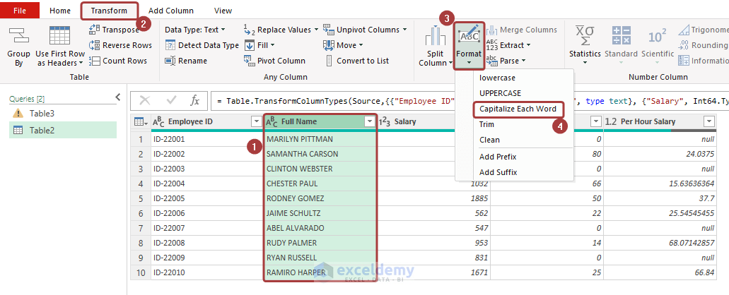
- We will get the names in the proper case.
- To remove the entire rows based on the blank cells in the Per Hour Salary column, click on the filter button and pick the Remove Empty option.
- Click OK.
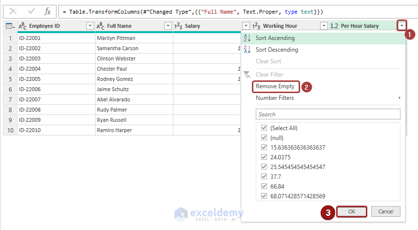
- We will get a filtered table with no rows with blank cells.
- Go to Home and click Close & Load from Close & Load.
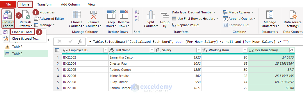
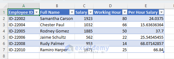
- We will get the filtered dataset in a new worksheet.
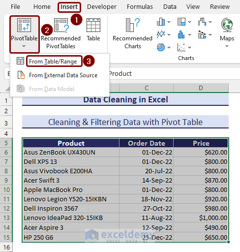
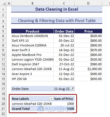
Method 23 – Cleaning and Filtering Data with a Pivot Table
- In order to create a pivot table, select the range of cells and go to the Insert tab.
- Click on Pivot Table from the ribbon and choose From Table/Range.
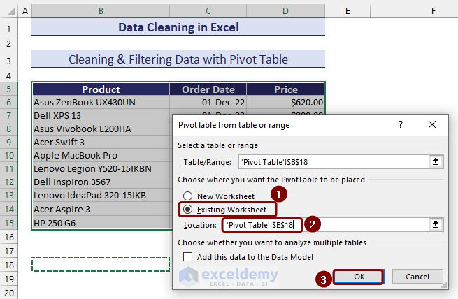
- Define the pivot table location from the PivotTable from table or range. It could be in the current worksheet or an entirely new worksheet.
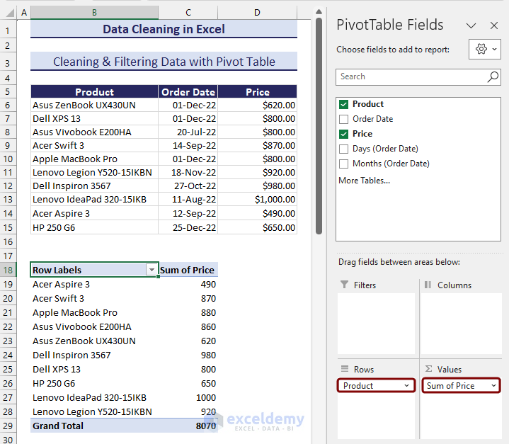
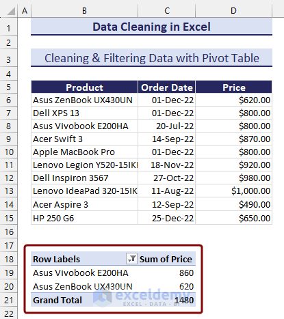
- Define rows and values. We have defined the products as rows and prices as values.
- To summarize the dataset with rows containing certain text, click on the filter button on the column header.
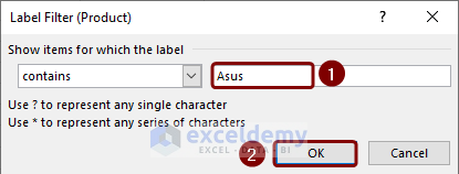
- Go to Label Filters and choose the Contains… option.
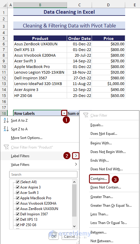
- Insert the specific word (i.e. Asus) based on what you want to filter the table and click on OK.
- The product with that specific text will be sorted.
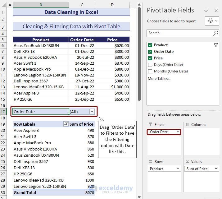
- To add Order Date as a parameter to filter the dataset, drag Order Date to the Filter section in PivotTable Fields.
- Pick a date as a filtering parameter.
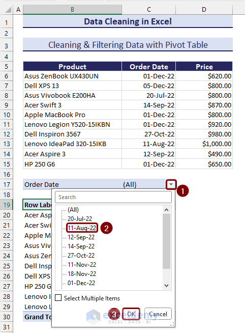
- We will get the pivot table.
Method 24 – Changing the Number Format into Percentage
- Divide the obtained value with the total value. We have applied the following formula to have the total obtained marks in decimal format:
=SUM(D8:F8)/$G$5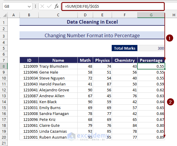
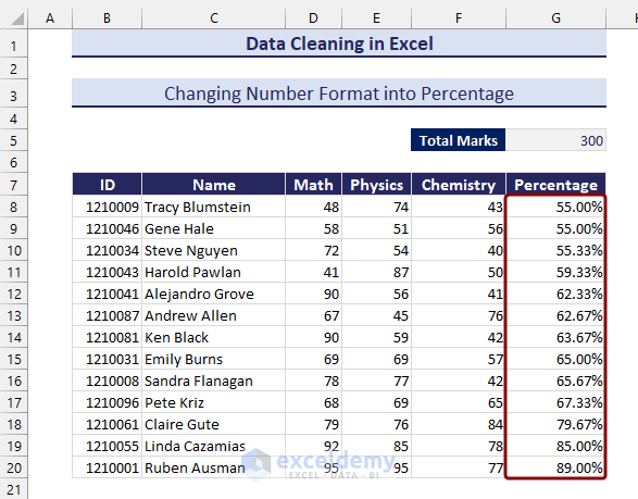
- Select all the decimal numbers and change the number format to Percentage from the Number Format option under the Home tab.
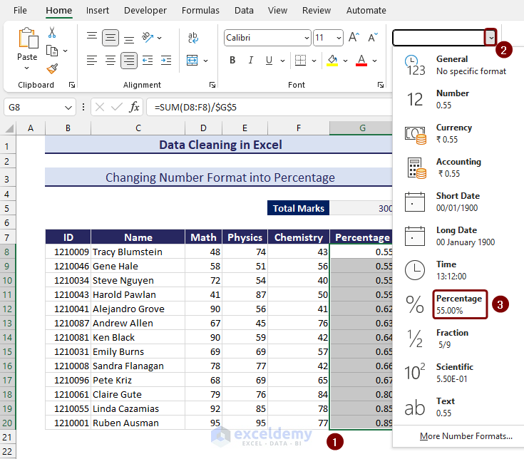
- We get the percentages.
Method 25 – Finding Maximum and Minimum Values
- Apply the following formula with the MAX function to find out the maximum value of a range:
=MAX(G7:G21)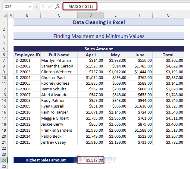
- You can use the following formula with the MIN function to find the minimum value from the defined range:
=MIN(G7:G21)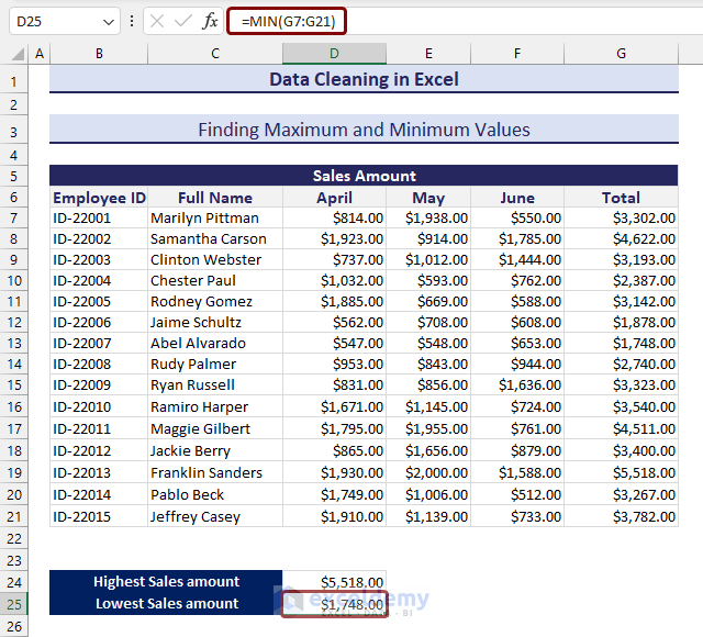
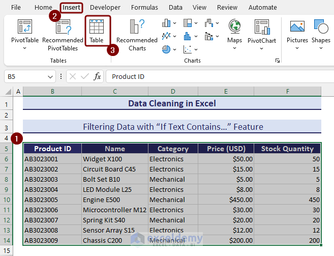
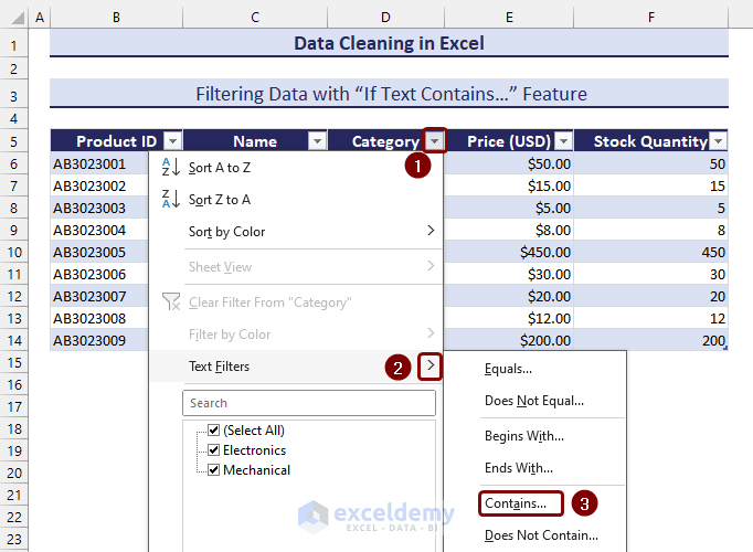
Method 26 – Filtering Data with the “If Text Contains…” Feature
The following dataset is categorized into electronics and mechanical categories. We will filter data that belong to the mechanical category.
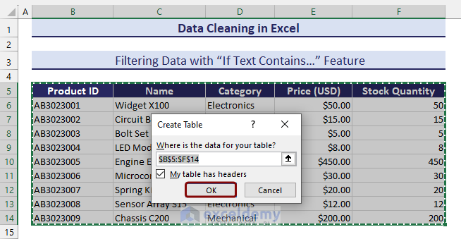
- Select a range of cells and click on Table from the Insert tab.
- Confirm the table range by clicking on OK.
- Click on the filter button from the column header.
- Select the Contains… option from Text Filters.
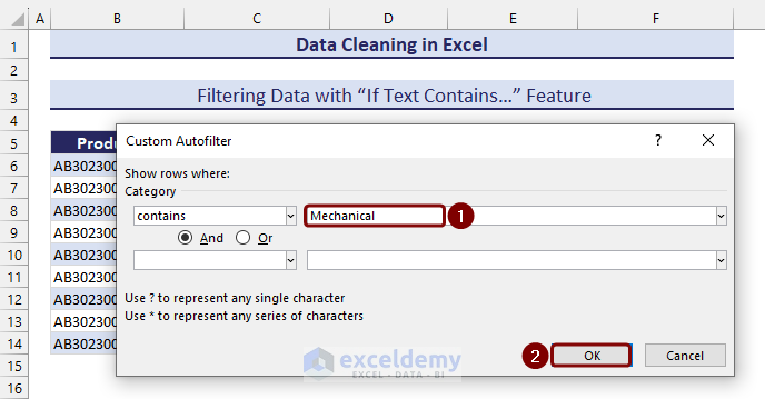
- Insert the specific text (i.e. Mechanical) on the contains category based on what you want to filter the dataset.
- Click on OK to finish the process.
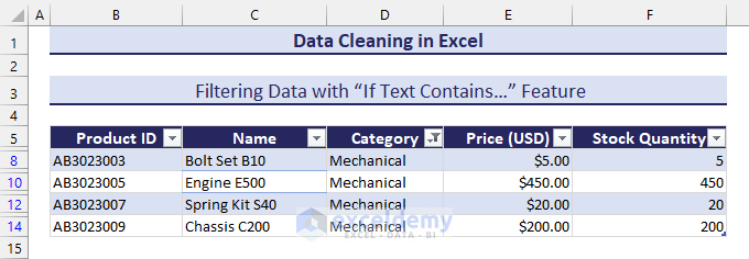
- We get the filtered table that contains a specific text.
Method 27 – Checking Data Types
The TYPE function will return an integer number based on the type of data according to the following table:
| Category | Return value |
| Number | 1 |
| Text | 2 |
| Logical Value | 16 |
| Error | 4 |
| Array | 64 |
- Apply the following formula with the TYPE function to check the data type:
=TYPE(F6)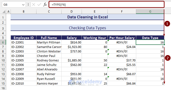
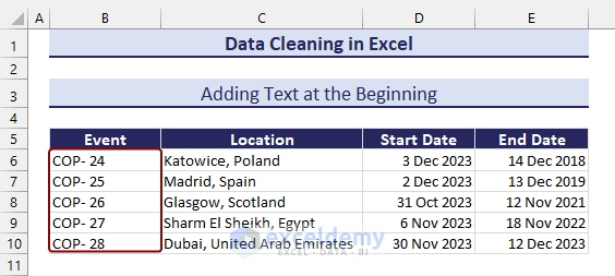
Method 28 – Adding Text at the Beginning
Column B under the Event header needs to be represented more clearly with additional “COP- “ text at the beginning.
- Use the following formula with the CONCATENATE function to add text at the beginning:
=CONCATENATE(“COP- “,B6)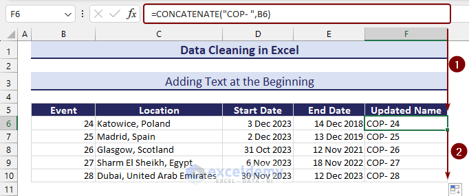
- Copy those updated values and paste as values in the desired location.
Method 29 – Adding Text at the End
In column E, under the Address header, we’ll add the country name USA for all state names at the end.
- Apply the following formula with the CONCAT function to add text at the end of a cell value:
=CONCAT(E6,"-USA")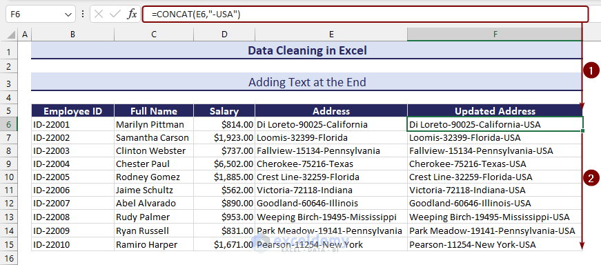
Method 30 – Inserting a Comma Before the Nth Character from Right
In column E under the Address header, we will insert a comma and a space.
- To insert a comma and a space before the 3rd character from the right, apply the following formula:
=LEFT(E6, LEN(E6) - 3)& ", " &RIGHT(E6, 3)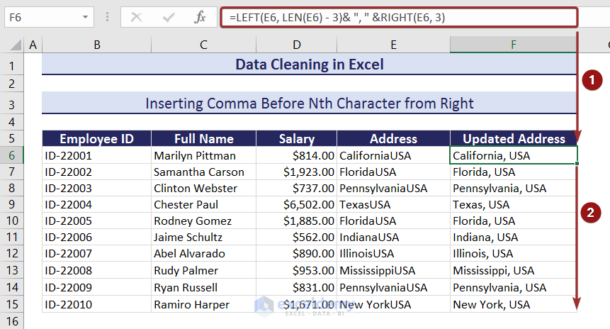
Method 31 – Removing Text Starting from a Particular Character
In column E under the Address header, we will remove the entire part after the comma portion, including that comma.
- Apply the following formula with the LEFT and SEARCH functions to remove text starting from a particular character:
=LEFT(E6,SEARCH(",",E6)-1)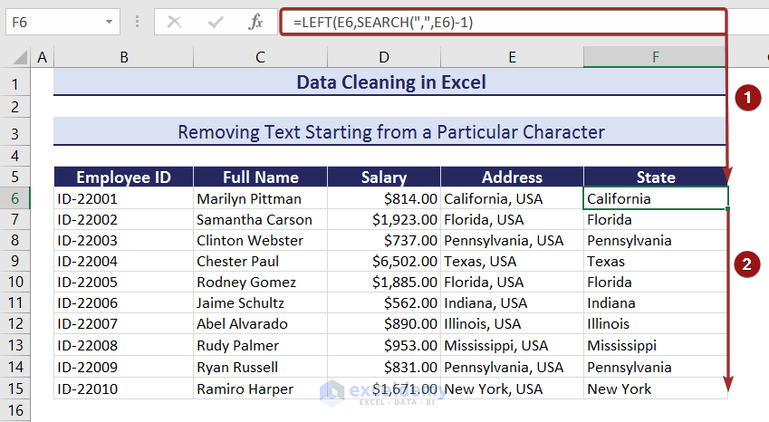
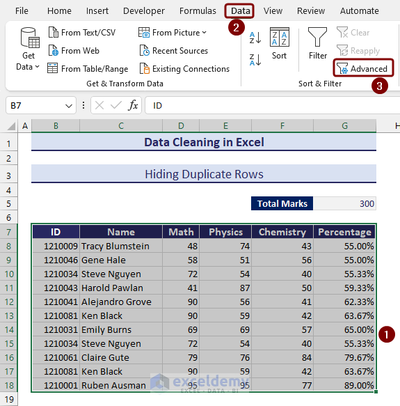
Method 32 – Hiding Duplicate Rows
- Select the range of data and go to the Data tab.
- Click on the Advanced options from the ribbon.
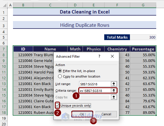
- From the Advanced Filter wizard, define the data range again in the Criteria range section and check the Unique records only box.
- Click on OK to finish the process.
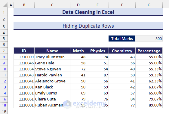
- We have the duplicate data hidden.
Method 33 – Using Add-ins
There are many websites that provide free add-ins that lessen our workloads to execute data cleaning in Excel. Some of the websites are listed below:
What Are the Challenges of Data Cleaning in Excel?
- There is a limitation in data size in Excel that can lead to difficulties while cleaning data.
- As data cleaning in Excel is a manual process, it is tedious, time-consuming, and prone to human error.
- Missing data can lead to a wrong prediction while cleaning data.
- Dealing with outliers is a very difficult and error-prone task.
- Excel can’t directly process unstructured data like images, audio, text documents, etc.
Download the Practice Workbook
Data Cleaning in Excel: Knowledge Hub
- How to Remove Numbers from a Cell in Excel
- How to Remove Outliers in Excel
- How to Remove Dotted Lines in Excel
- How to Remove Compatibility Mode in Excel
- How to Remove Value in Excel
- How to Remove 0 from Excel
- How to Remove Panes in Excel
- How to Remove Drop Down Arrow in Excel
- How to Remove HTML Tags from Text in Excel
- How to Remove Partial Data from Multiple Cells in Excel
- Using Excel to Clean and Prepare Data for Analysis
- How to Clean Up Raw Data in Excel
- How to Clean Survey Data in Excel
- 19 Practical Data Cleaning Techniques in Excel
- How to Do Automated Data Cleaning in Excel
- How to Use Macro to Clean Up Data in Excel
<< Go Back To Learn Excel
Get FREE Advanced Excel Exercises with Solutions!

Dear Naimul Hasan Arif and Nehad Ulfat,
I hope this message finds you well. My name is AKhtar Khilji, and I’m reaching out to express my sincere appreciation for the outstanding training blog you have crafted to assist users in addressing data cleaning challenges.
Currently, I am conducting a training program on Excel through a nonprofit organization, focusing on empowering the youth of marginalized communities. I was deeply impressed by the quality of your training material and would like to request your permission to utilize the exercises from your blog. Of course, I will ensure proper attribution by mentioning “Excel Dummy” along with the web address. Furthermore, I intend to share the reading material with the trainees to enhance their learning experience.
Thank you so much for considering my request. Your generosity will undoubtedly contribute to the success of this educational initiative.
Best regards,
AKhtar Khilji from Pakistan
Dear AKhtar Khilji,
I hope this message finds you well too. Thank you very much for your kind words and your interest in using the training material from my blog for your nonprofit Excel training program. I’m thrilled to hear that you found the content helpful and that it will be used to empower the youth of marginalized communities in Pakistan.
I’m more than happy to grant you permission to utilize the exercises from the blog for your educational initiative. Please feel free to mention “ExcelDemy” along with the web address to provide proper attribution. It’s wonderful to know that the material will be shared with the trainees to enhance their learning experience.
If you have any specific requests or need further assistance with anything related to the training material, please don’t hesitate to reach out. I’m here to support your efforts in any way I can.
Wishing you great success with your Excel training program and the empowerment of the youth in marginalized communities.
Best regards,
ExcelDemy