In Excel, it is a common thing that you need to clean up your raw data. You might need to remove duplicates or find and replace some specific cells or change the casings of your letters and so on. In this article, I will show you the 10 coolest and easiest ways to clean up raw data in Excel.
10 Ways to Clean Up Raw Data in Excel
Go through the full article below to learn and apply 10 methods for cleaning up raw data in Excel. 👇
1. Remove or Highlight Duplicate Cells
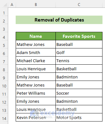
Say, you have a dataset of 10 persons’ names and favorite sports. Now, there might be some duplicate values in your dataset. You can remove these duplicate cells in two ways described below. 👇
1.1 Remove Duplicates
You can directly remove duplicate cells using the Remove Duplicates tool. Follow the steps below to do this. 👇
📌 Steps:
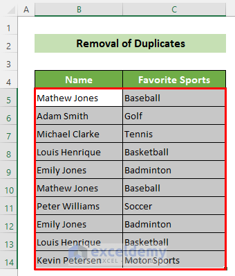
- First and foremost, select all the cells that you want to check if any duplicate values are present.
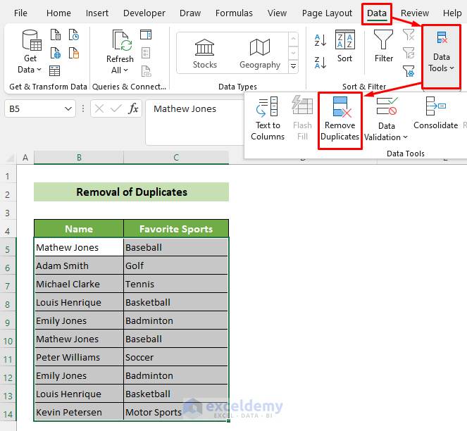
- Next, go to the Data tab >> Data Tools group >> Remove Duplicates tool.
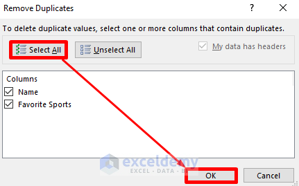
- At this time, the Remove Duplicates dialogue box will appear. Now, click on the Select All button and subsequently, click on the OK button.
- Now, you can see a Microsoft Excel dialogue box will appear notifying you of the changes. Click on the OK button.
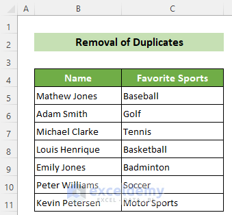
Finally, all your duplicate values are removed. And, the result sheet should look like this. 👇
1.2 Highlight Duplicates
You can also highlight duplicates using conditional formatting rather than deleting them. Go through the steps below to do this. 👇
📌 Steps:
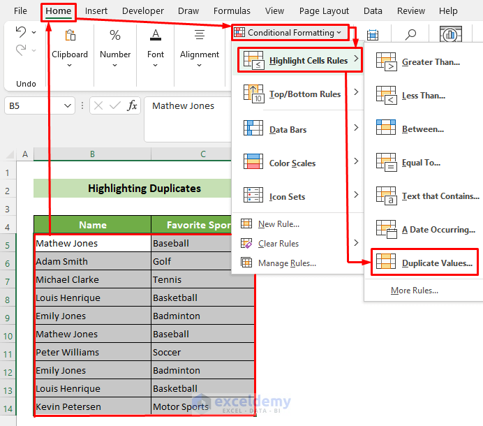
- Initially, select your dataset. Subsequently, go to the Home tab >> Styles group >> Conditional Formatting tool >> Highlight Cells Rules >> Duplicate Values…
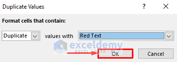
- As a result, the Duplicate Values dialogue box will appear. Here, you can choose the format in which you want to see the duplicate values. For doing this, click on the downward arrow beside the values with option. Let’s choose the Red text option from the listed options.
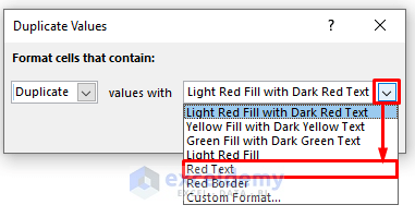
- Finally, click on the OK button.
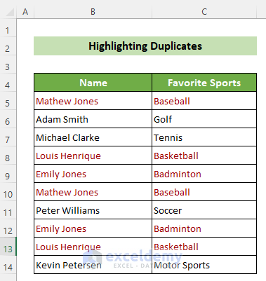
Thus, you can see your duplicate values are formatted as red text now. For instance, the result sheet should look like this. 👇
Read More: Using Excel to Clean and Prepare Data for Analysis
2. Find and Fill All Blank Cells
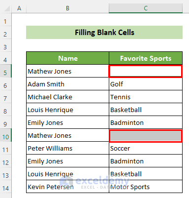
You can find and fill all the blank cells using the Find & Replace tool in Excel. Suppose, you have a data set where you have 10 person’s names and respective favorite sports. Two of the cells are blank and you want to fill these cells with the appropriate values. Follow the steps below to accomplish this. 👇

📌 Steps:
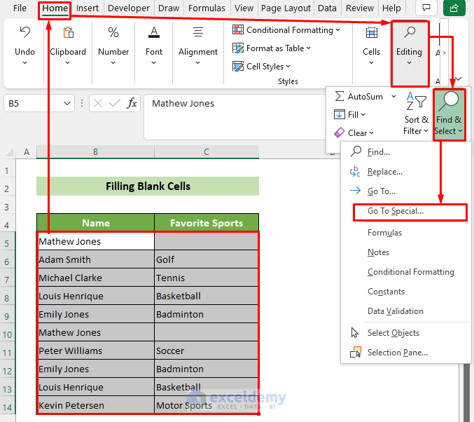
- Firstly, select your dataset. Following, go to the Home tab >> Editing group >> Find & Select tool >> Go to Special… option from the dropdown list.
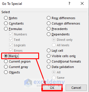
- At this time, the Go to Special dialogue box will appear. Put the radio button on the Blanks option and click on the OK button.
- As a result, all the blank cells of your dataset will be selected.
- Now, write the value that you want to insert inside the blank cells. Press Ctrl+Enter.
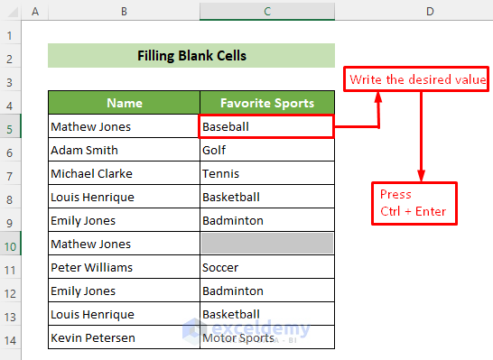
Thus, all the blank cells will have the same value now. And, the result sheet should look like this. 👇

Note:
If you press the Enter button instead of the Ctrl + Enter, then you have to write values in each individual blank cell. Here, only the active cell will have the value at each Enter button press.
Read More: How to Clean Survey Data in Excel
3. Find & Replace in Specific Cells
3.1 Find & Replace a Character (e.g. Parentheses)
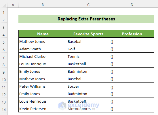
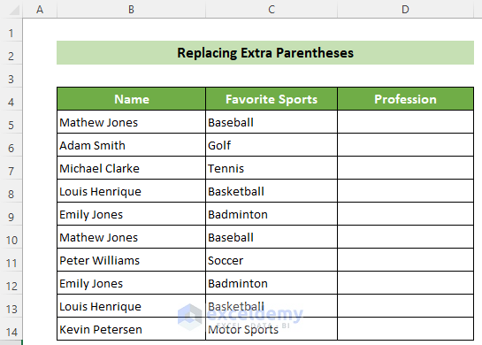
Now, you can see, that you have another column with the previous columns which is Profession. But, there is no valid profession in the column cells, rather there are parentheses by default. Now, you can remove these parentheses very easily by following the simple steps below. 👇
📌 Steps:
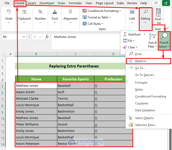
- First, select your dataset. Subsequently, go to the Home tab >> Editing group >> Find & Select tool >> Replace… option from the listed options.
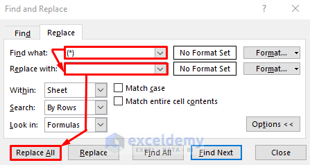
- As a result, the Find and Replace window will appear now. Subsequently, insert (*) inside the Find what: text box and insert a space inside the Replace with: text box. Finally, click on the Replace All button.
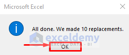
- At this time, you will see a Microsoft Excel dialogue box pops up and notifying you of the changes made. Click on the OK button.
Finally, you can see that all the parentheses of your dataset have been substituted by a space. For example, the result sheet would look like this. 👇
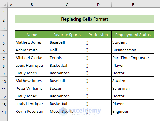
3.2 Find & Replace Cells Format
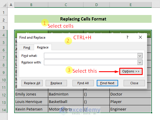
Now, suppose you have a dataset of 10 people’s Names, Favourite Sports, Professions, and Employment Status columns. Some data are in a 12-size font and in bold format. Now, if you want to find the formatted cells and replace the format with some other format, follow the steps below. 👇
📌 Steps:
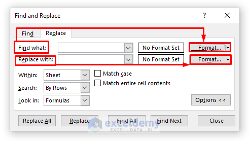
- First and foremost, select your dataset. Next, press the Ctrl + H button. This will bring up the Find and Replace dialogue box. Following, click on the Options > > button from the dialogue box.
- At this time, choose the format that you want to find by accessing the Find what: option’s Format… button. And, select your desired format from the Replace with: options Format… button.
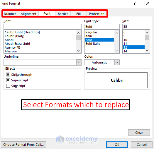
- As we want to find the 12-size Bold format text, we chose the following options from the Find Format window.
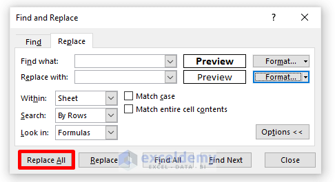
- Last but not least, after choosing the find format and replace format, click on the Replace All button.
- At this time, you will see that a Microsoft Excel dialogue box will appear. It will notify you about the changes that have been made. Now, click on the OK button.
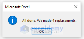
Thus, you can find and replace the formats of your dataset. The final outcome should look like this. 👇
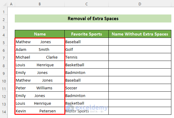
4. Remove Extra Spaces
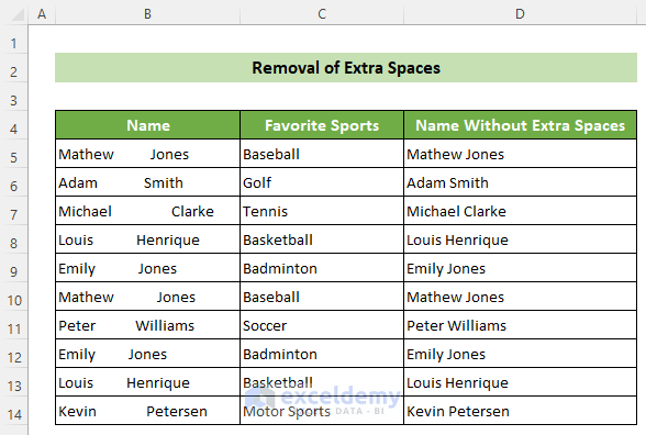
Another way to clean up raw data in Excel is to remove the extra spaces. Sometimes, it might happen that you have faced unnecessary spaces in your cell. Suppose, in your dataset, there are unwanted spaces in the Name column. Now, you can remove these extra spaces using the TRIM function following the steps given below. 👇
The TRIM function is an Excel function that is used to remove extra spaces from a cell. It keeps only one space between each word. It has only one argument: the text. In this argument, you need to put in the text or the cell reference at which you want to remove extra space.
📌 Steps:
- Firstly, select the D5 cell and write the following formula.
=TRIM(B5)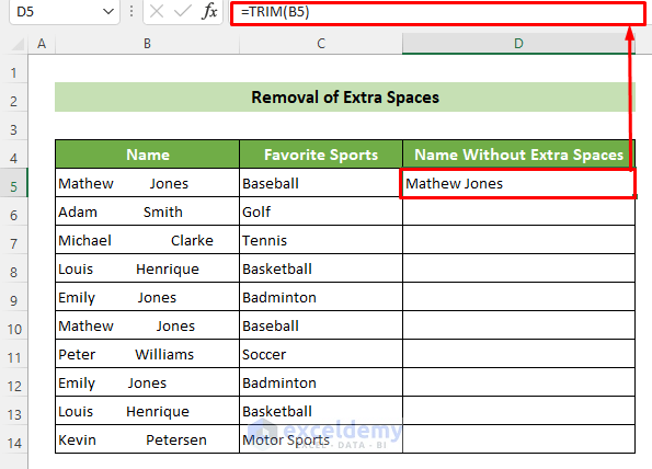
- As a result, the unnecessary spaces of the B5 column will be removed. Now, put your cursor in the bottom-right position of your cell. Consequently, a fill handle will appear. Drag it downward.
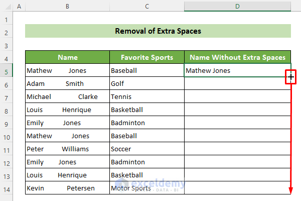
As a result, all the extra spaces of B5:B14 cells will be removed in the D5:D14 cells. For a quick look, the result sheet will look like this. 👇
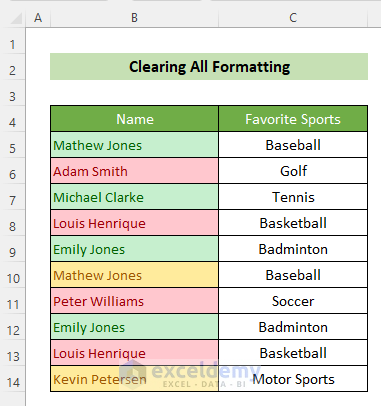
5. Clear All Formatting
Now, suppose you have a default format for your dataset, but you want to clear all this default formatting and make a new format for the dataset according to your desire. To clear the formatting, follow the steps below. 👇
📌 Steps:
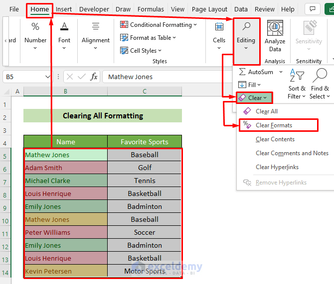
- At the very beginning, select all the cells of your dataset. Subsequently, go to the Home tab >> Editing group >> Clear tool >> Clear Formats option.
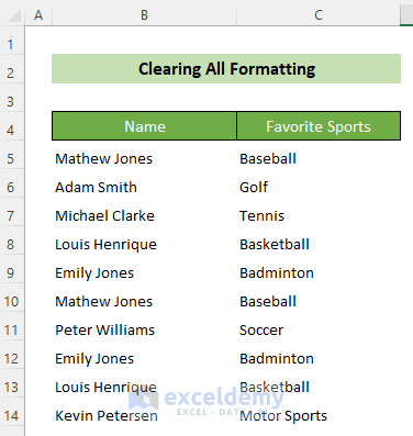
Thus, you can see now that there is no formatting of your dataset anymore. It has gone back to Excel’s default format of a dataset and the result sheet will look like this. 👇
Read More: 19 Practical Data Cleaning Techniques in Excel
6. Check and Identify Errors
To clean up raw data in Excel, another thing might happen. That is, suppose, you have a large dataset and you have some errors in your dataset. Now, you can find the errors in the following ways. 👇
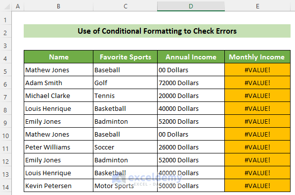
6.1 Use Conditional Formatting
You can use conditional formatting to accomplish this. Follow the steps below to do this. 👇
📌 Steps:
- First and foremost, select your dataset. Next, go to the Home tab >> Conditional Formatting tool >> New Rule… option.
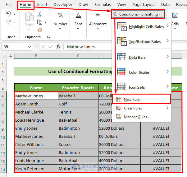
- Asa result, the New Formatting Rule window will appear. Select the option Format only cells that contain. Following, choose the option Errors from the Format only cells with: dropdown list. Next, click on the Format… button.
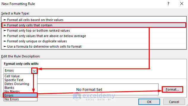
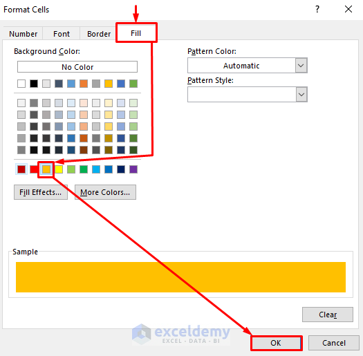
- At this time, the Format Cells window will appear. Here, go to the Fill tab and choose your desired color for your error cell highlighter. Click on the OK button.
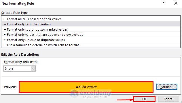
- Now, you will see the New Formatting Rule window has come again and it is showing you the Preview of your error cell format. Finally, click on the OK button.
Thus, the errors of your dataset are highlighted now successfully. And, It should look like this now. 👇
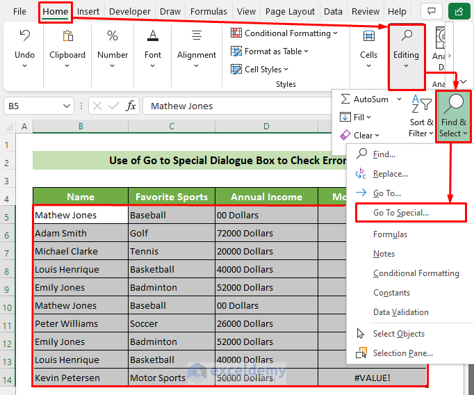
6.2 Use Go To Special Dialogue Box
Besides, you can also use the Go to Special dialogue box to find your errors. Just follow the steps below to achieve this. 👇
📌 Steps:
- First, select your dataset. Subsequently, go to the Home tab >> Editing group >> Find & Select tool >> Go To Special… option from the dropdown list.
- At this time, the Go To Special dialogue box will appear. Next, put the radio button on the Formulas option. Following, deselect all the options without the Errors option. Finally, click on the OK button.
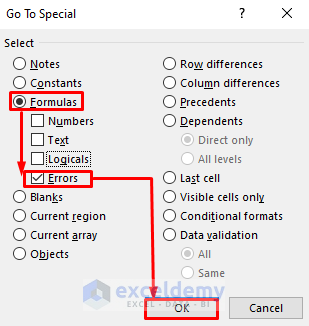
As a result, you can find all the errors in your dataset as you can see that all of them are selected at a time. For instance, the outcome will look like this. 👇

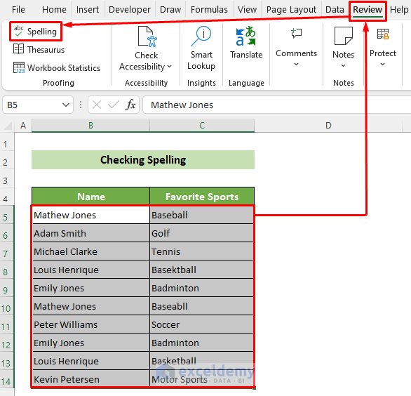
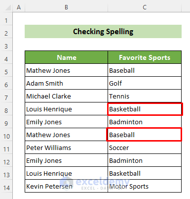
7. Check Spelling
You can also check if you have any spelling errors in your dataset. Follow the steps below to achieve this. 👇
📌 Steps:
- Initially, select the dataset. Next, go to the Review tab >> Spelling tool.
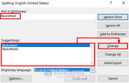
- As a result, the Spelling window will appear. It will show your spelling error and give you suggestions for the solution. Following, select the suggestion that you actually are looking for and click on the Change button.
- After a full spelling check of your dataset, a Microsoft Excel dialogue box will appear showing you the message of spelling check completion. Click on the OK button.

Thus, all cells of your dataset are free from spelling errors now. Your outcome should look like this. 👇
Spell Checking Shortcut: F7
8. Change Case of Letters
In order to clean up raw data in Excel, you can change the cases of your letters in your dataset too.
8.1 Change to Uppercase
To make your letters uppercase, you can use the UPPER function. Follow the steps below to achieve this. 👇
The UPPER function is an Excel function that uppercases the letters of a cell. It has only one argument: the text. It takes in the text and makes it uppercased.

📌 Steps:
- Firstly, select the D5 cell where you want to put the uppercased name. Following, write the formula below.
=UPPER(B5)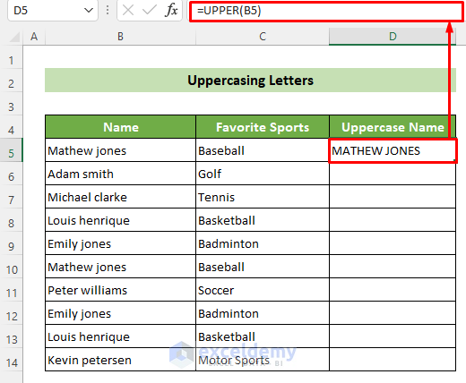
- As a result, you will get the uppercased text of the B5 cell. Now, put your cursor in the bottom right position of your cell, and consequently, a black fill handle will appear. Drag it downward to copy the formula for all the cells.
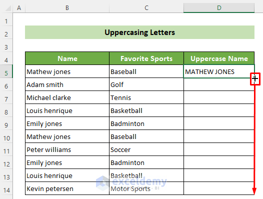
Thus, all your names will be in uppercase now. For instance, the outcome should look like this. 👇

8.2 Change to Lowercase
Besides, you can lowercase the letters of a cell using the LOWER function. Use the steps below to do this. 👇
The LOWER function is an Excel function that lowercase the letters of a text. It has only one argument, that is text. It takes the text and makes it lowercase.

📌 Steps:
- Initially, click on the D5 cell and insert the following formula.
=LOWER(B5)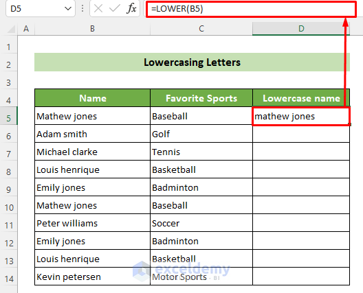
- Now, you will get the B5 cell as lowercase text. Following, place your cursor in the bottom right position of your cell. Consequently, the fill handle will appear. Now, drag it downward to copy the formula for all the cells below.

Consequently, you can lowercase the names of your dataset. And, the outcome should look like this. 👇

8.3 Change to Propercase
Moreover, you can propercase your dataset using the PROPER function. Go through the following steps to do this. 👇
The PROPER function is an Excel function propercases words of a text. It requires only one argument: text. IN this argument you need to give the cell reference or text that you want to propercase.

📌 Steps:
- Firstly, select cell D5 and write the following formula in the formula bar.
=PROPER(B5)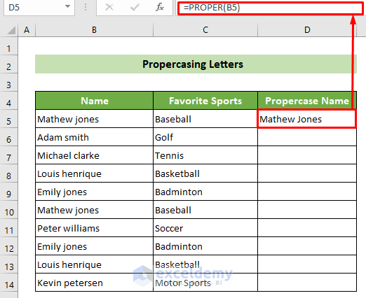
- As a result, you can get the propercase name of the first person. Next, place your cursor in the bottom right position of your cell. You can see a fill handle will appear. Drag it downward to copy the formula for all the cells.
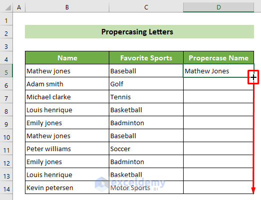
Thus, you can propercase every name of your dataset. For example, it would look like this. 👇

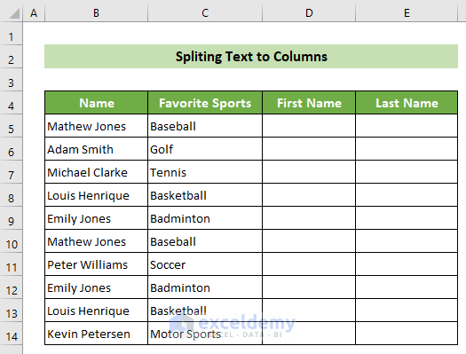
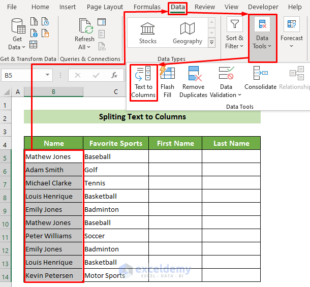
9. Split Text in One Cell to Multiple Columns
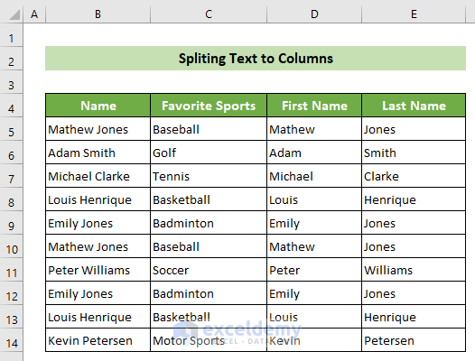
Another thing, you can split your text to columns for various purposes. It is very handy sometimes. Say, you have a dataset of the full names of several persons. Now, you can split text to column and so get their first and last name in different columns.
📌Steps:
- First and foremost, select all the names of your dataset that is B5:B14 here. Subsequently, go to the Data tab >> Data Tools group >> Text to Columns tool.
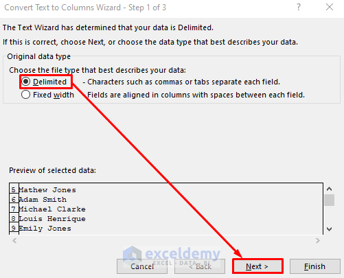
- As a result, the Convert Text to Columns Wizard dialogue box will appear. Put the radio button on the Delimited option and click on the Next button.
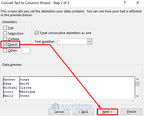
- Following, another Convert Text to Columns Wizard dialogue box will appear. Here, tick only the option Space and click on the Next button afterward.
- Last but not least, another Convert Text to Columns Wizard dialogue box will appear. Choose the Column data format as General and insert your destination at the Destination text box. Finally, click on the Finish button.
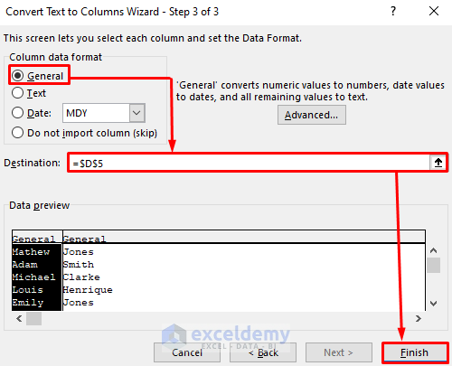
Thus, you can see that you have split the B column cell text to D and E columns. And the result sheet will look like this. 👇
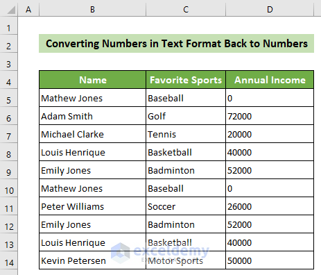
10. Convert Numbers in Text Format Back to Numbers
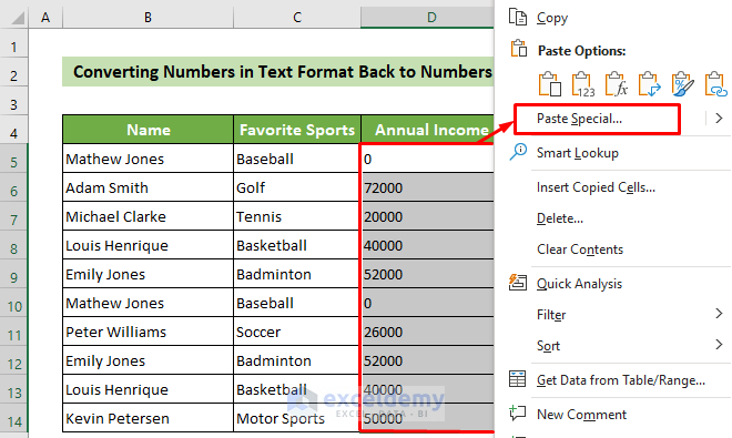
Now, suppose you have the dataset as Name, Favorite Sports, and Annual Income Columns. But, the Annual Income column’s data are left-aligned which means they are in the text format. It will create problems when calculating with these cells. Now, you can convert these numbers back to number format through the following steps. 👇
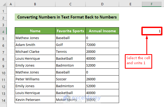
📌 Steps:
- Initially, click on a random cell and write 1. Say, we select the F4 cell and write 1.
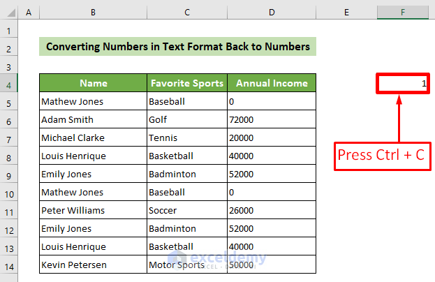
- Now, copy the F4 cell by pressing the Ctrl+C.
- Next, select the D5:D14 cell where you want your conversion. Subsequently, right-click on your mouse and choose the Paste Special… option from the context menu.
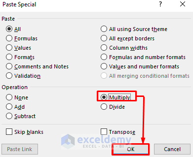
- As a result, the Paste Special window will appear. Following, choose the Multiply option from the Operation group. Finally, click on the OK button.
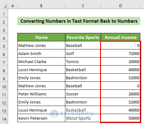
Thus, you can see that the Annual Income cell values are right-aligned now. So, you can tell they are in number format now. As an example, the result sheet would look like this. 👇
Download Practice Workbook
You can download and practice from our workbook here.
Conclusion
In brief, in this article, I have shown you the 10 most effective and necessary ways to clean up raw data in Excel with examples. I would suggest you read the full article and practice on your own from our given practice workbook. It would definitely enhance your knowledge and expertise regarding this objective. I hope you find this article helpful and informative. Furthermore, if you have any queries or recommendations, feel free to comment here.
Related Articles
- How to Remove Partial Data from Multiple Cells in Excel
- How to Do Automated Data Cleaning in Excel
- How to Use Macro to Clean Up Data in Excel
<< Go Back To Data Cleaning in Excel | Learn Excel
Get FREE Advanced Excel Exercises with Solutions!
