Method 1 – Remove Duplicate Rows
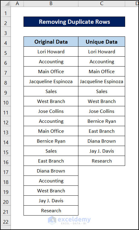
Here’s a sample dataset that contains duplicate rows.
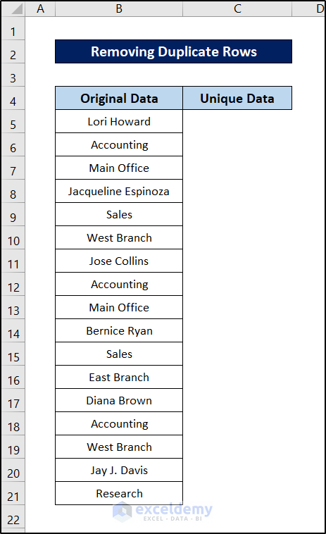
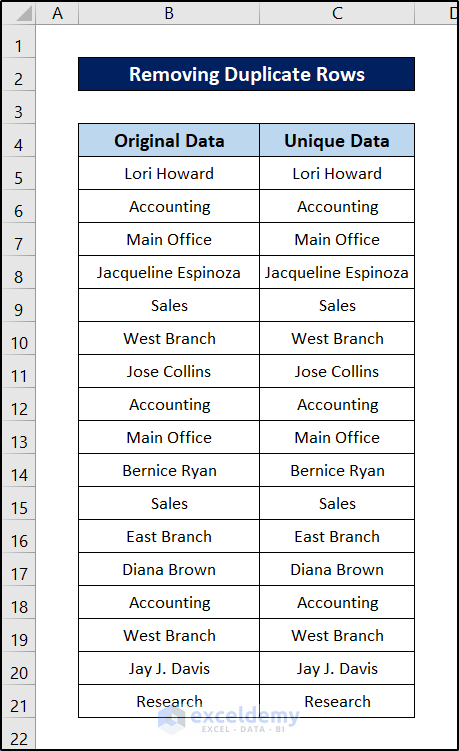
Let’s replicate the column and remove the duplicates to compare them later on.
Steps:
- Select the column you want to remove the duplicates from.
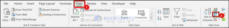
- Go to the Data tab on your ribbon.
- Select Remove Duplicates from the Data Tools group.
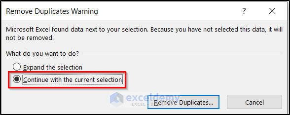
- Select the Continue with the current selection option in the pop-up box and click on Remove Duplicates.
- Click on OK.
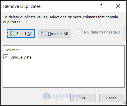
- This will remove all the duplicates from the selection.
Read More: How to Clean Survey Data in Excel
Method 2 – Highlight Duplicate Values
Utilizing Conditional Formatting
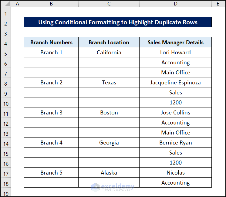
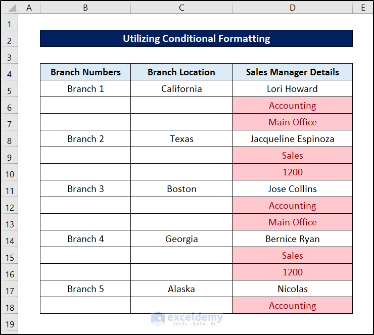
We’ll use the following dataset.
Steps:
- Select the cells that we want to highlight. In this case, it is D5:D18.
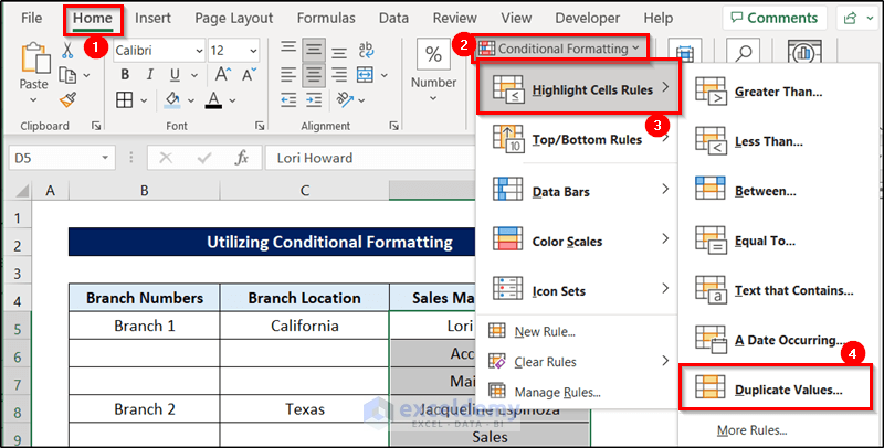
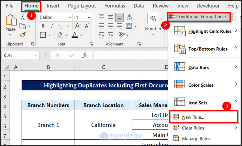
- Go to Home and choose Conditional Formatting.
- Go to Highlight Cells Rules and select Duplicate Values.
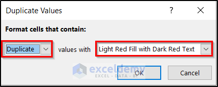
- A Duplicate Values window will appear.
- Choose Duplicate.
- Select any color options after values with. We have selected Light Red Fill with Dark Red Text.
- The duplicate values in the D column are highlighted.
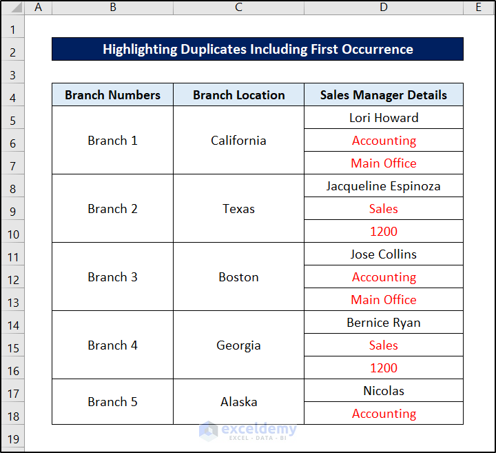
Highlighting Duplicates Including First Occurrence
Steps:
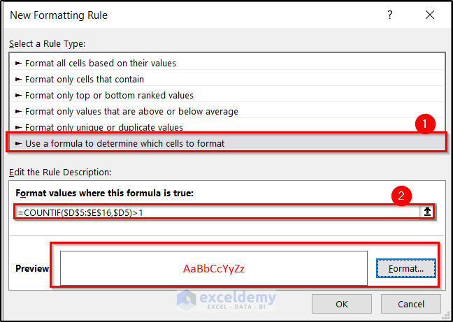
- Go to the New Formatting Rule window in Conditional Formatting
- Choose Use a formula to determine which cells to format.
- Use the following formula in the formula box.
=COUNTIF($D$5:$E$16,$D5)>1
- The D column is highlighted for duplicates, including the first occurrences.
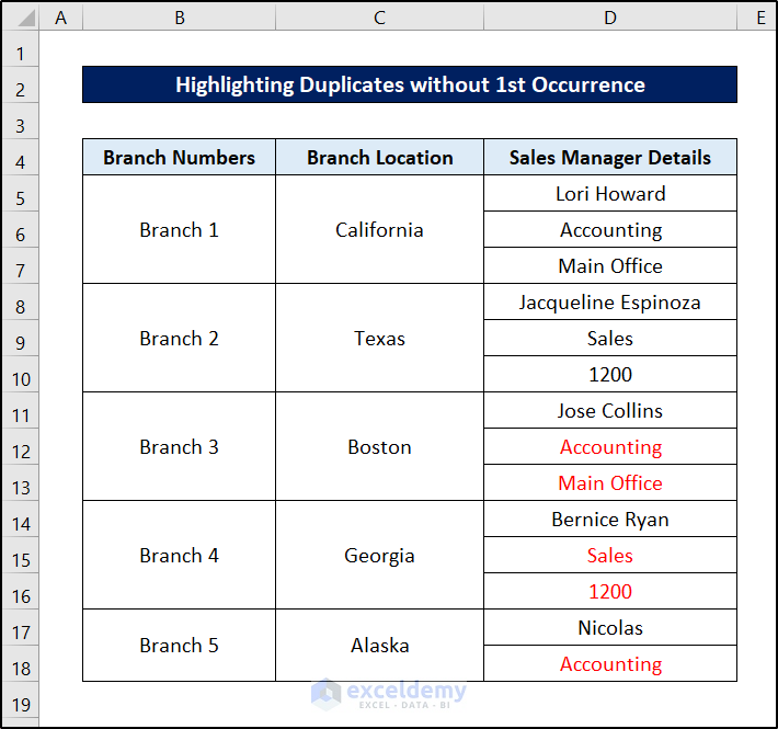
Highlighting Duplicates Excluding First Occurrence
Steps:
- Go to New Formatting Rule through the Conditional Formatting option.
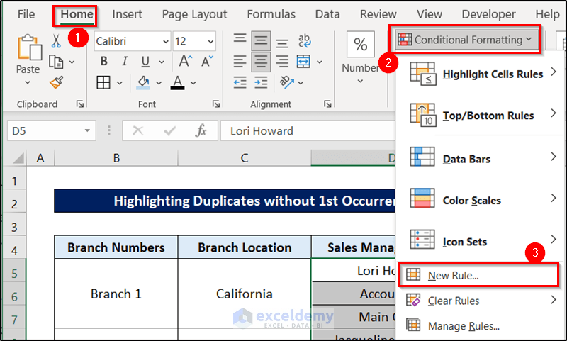
- Select Use a formula to determine which cells to format.
- Use the following formula in the formula box.
=COUNTIF($D$5:$D5,$D5)>1
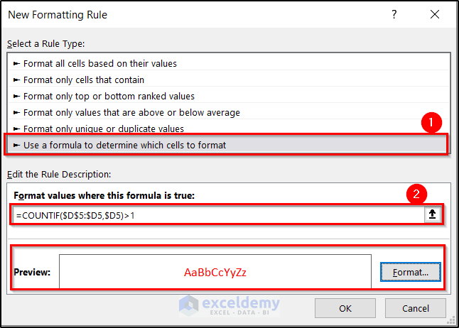
- Click OK for the result.
Read More: How to Clean Up Raw Data in Excel
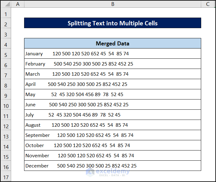
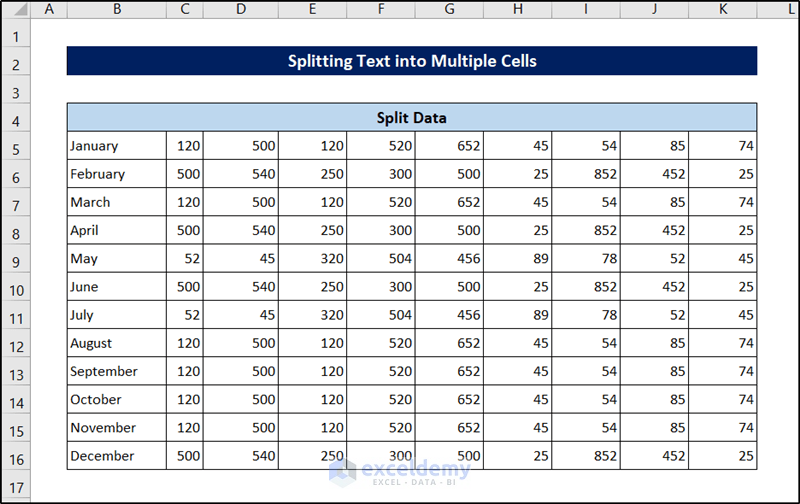
Method 3 – Split Text into Multiple Cells
Here’s a dataset where each cell has multiple values that need to be split.
Steps:
- Select the range you want to split text from.
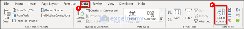
- Go to the Data tab on your ribbon.
- From the Data Tools group, select Text to Columns.
- Select Delimited in the next box.
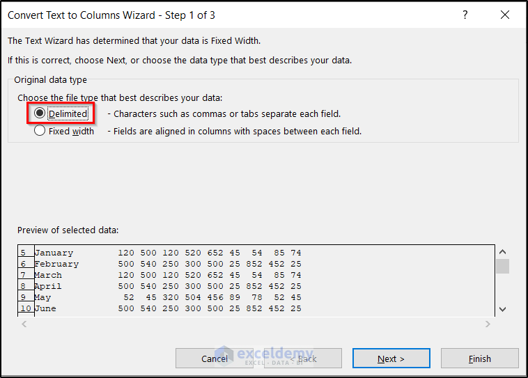
- After clicking on Next, another box will appear.
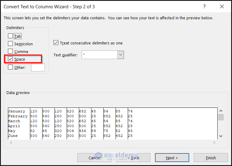
- Select Space under Delimiter options as the text is divided by spaces.
- Click on Next.
- Click on Finish.
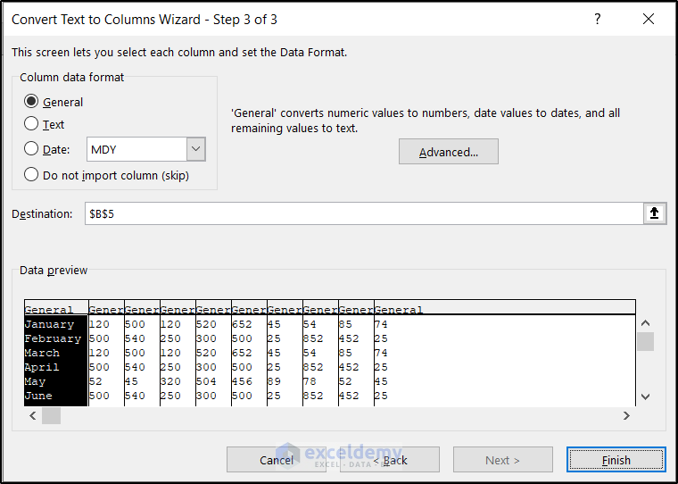
- The text will be split.

- Let’s make some modifications to make the data more presentable.
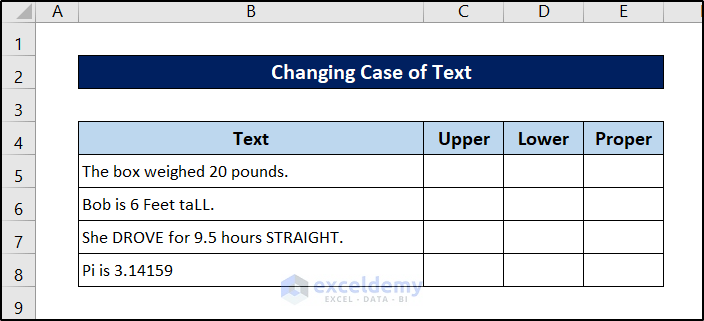
Method 4 – Transforming Data with Formulas
The three formulas to change text are:
UPPER: This formula converts the text to ALL UPPERCASE.
LOWER: This formula converts the text to all lowercase.
PROPER: This one converts the text to Proper Case (the first letter in each word will be capitalized, as in a proper name).
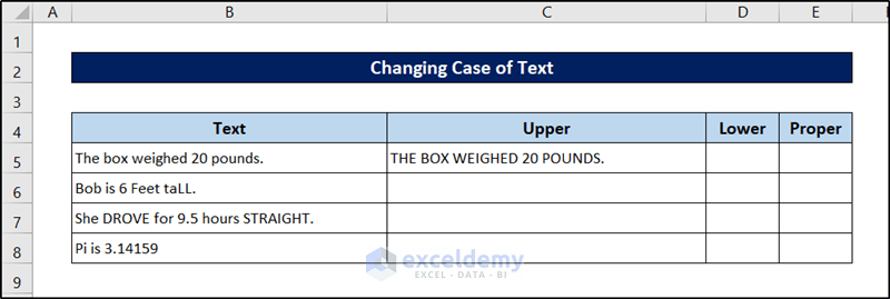
We will use the following dataset.
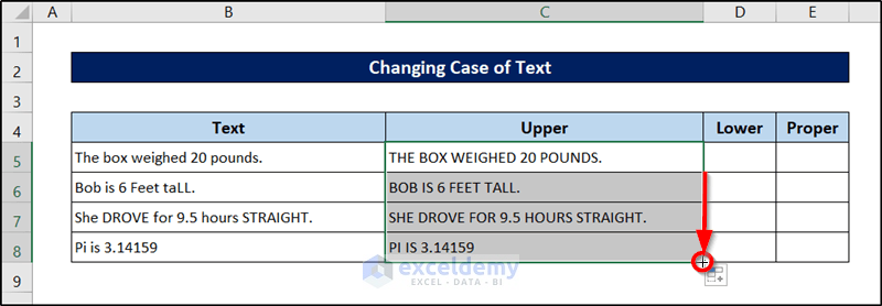
Changing to Upper Case
Steps:
- Select cell C5.
- Use the following formula in it.
=UPPER(B5)
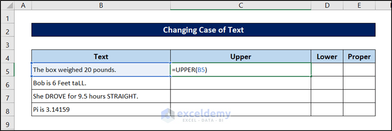
- Press Enter.
- Select the cell again and click and drag the fill handle icon down to fill the rest of the cells with the formula.
Changing to Lower Case
Steps:
- Select cell D5.
- Use the following formula in it.
=LOWER(B5)
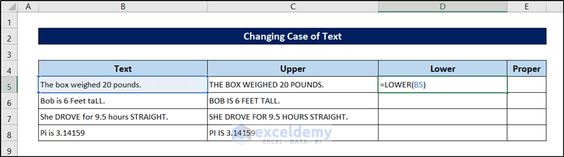
- Press Enter.
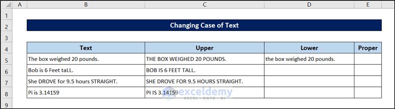
- Select the cell again and click and drag the fill handle icon down to fill the rest of the cells with the formula.
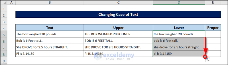
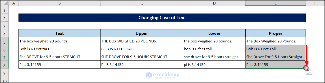
Changing to Proper Case
Steps:
- Select cell E5.
- Use the following formula in it.
=PROPER(B5)
- Press Enter.
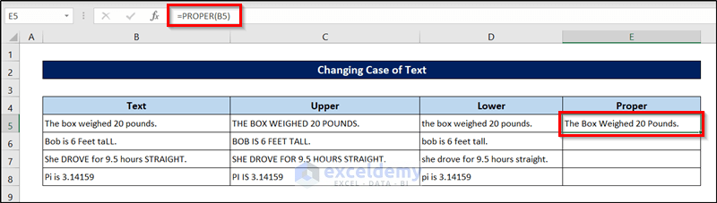
- Select the cell again and click and drag the fill handle icon down to fill out the rest of the cells.
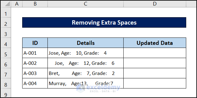
Method 5 – Remove Extra Spaces
We have a dataset where the values have extra spaces between them.
Using the TRIM Function
The TRIM function removes all leading and trailing spaces from a text and replaces multiple spaces with a single space.
Steps:
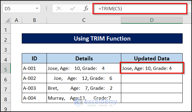
- Add a column D named Updated Data to show the results.
- Click on cell D5.
- Type =TRIM and select Cell C5 in the first argument. Close the parenthesis.
- The formula becomes:
=TRIM(C5)
- Press Enter.
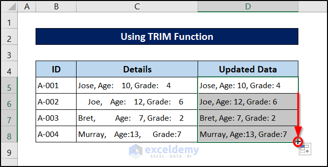
- Drag the Fill Handle icon down to the last cell.
Using the Find & Replace Feature:
Steps:
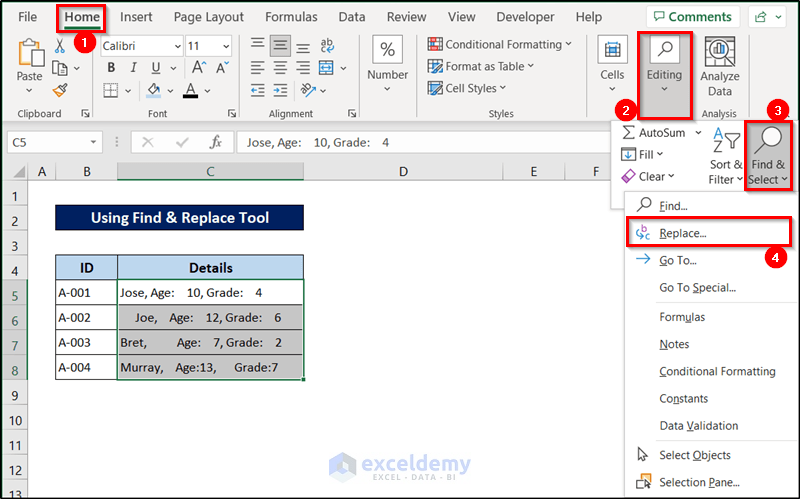
- Select the data from where you want to remove the extra spaces.
- Go to the Home tab.
- From the Editing command, go to the Find & Select feature.
- Select Replace from the drop-down list.
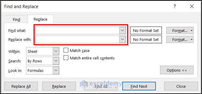
- You will get a dialog box.
- Type a blank space in the Find what field.
- Keep the Replace with box empty.
- Click Replace All.
- You’ll get a Pop-Up showing the number of replacements.
- Click OK.
- Click Close on the dialog box.
- Here’s the result.
Method 6 – Remove Strange Characters
You can use the CLEAN function to remove all non-printing characters from a text.
If the data is in cell A2, use this formula:
=CLEAN(A2)
The CLEAN function sometimes may miss some non-printing Unicode characters. It’s programmed to remove the first 32 non-printing characters in the 7-bit ASCII code. Browse the Excel Help system for information on how to remove the non-printing Unicode characters.
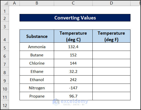
Method 7 – Convert Values
Let’s look at a dataset of temperatures that we need to convert between Celsius and Fahrenheit.
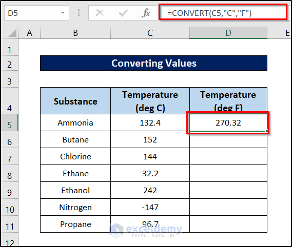
Steps:
- Select the output cell D5.
- Use the following formula:
=CONVERT(C5,"C","F")
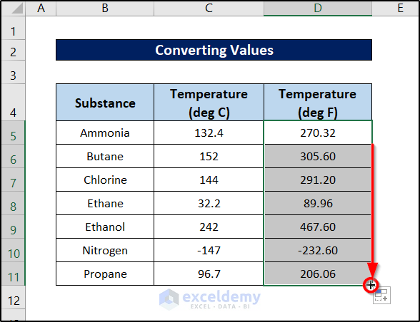
- Press Enter.
- Click and drag the fill handle icon to the end of the column to convert all values.
For other unit conversions, check out this article.
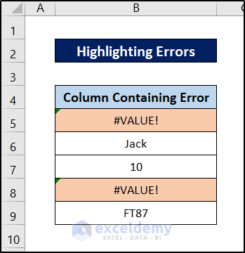
Method 8 – Highlight Errors
Suppose we have a dataset with some errors in some cells. We will highlight them with conditional formatting and the Go to Special feature.
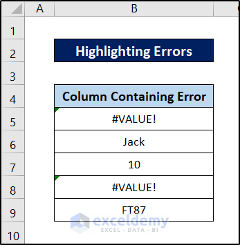
Steps:
- Select the whole dataset and click New Rule from the Conditional Formatting options.

- Choose Format Only cells that contain and select Errors from the drop-down list.
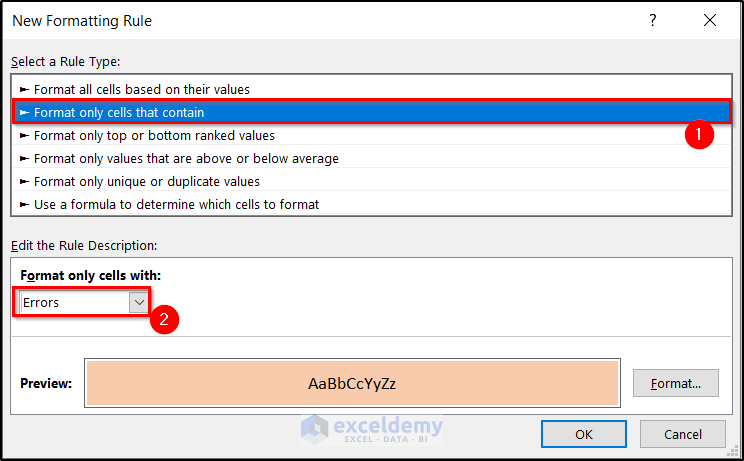
- Click on OK.
- Excel highlighted the error values.
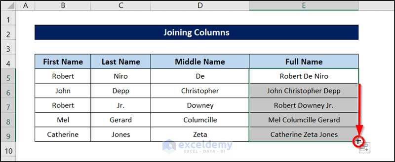
Method 9 – Join Columns
We’ll combine the first, middle, and last names in a single value for each entry in the list.
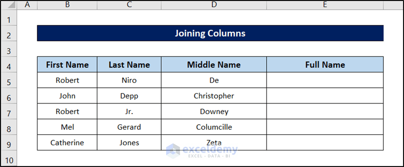
Steps:
- Select cell E5.
- Use the following formula.
=B5&" "&D5&" "&C5
- Press Enter.
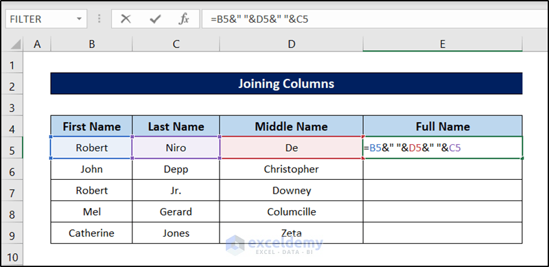
- Click and drag the fill handle icon to the end of the column to replicate the formula for the rest of the cells.
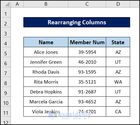
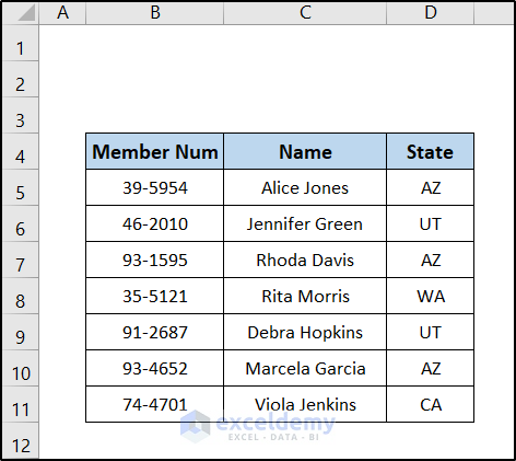
Method 10 – Rearrange Columns
Here’s a sample dataset where we’ll rearrange some columns.
Steps:
- Select the column you want to move by clicking on the column header.
- Cut the column using either the context menu or pressing Ctrl + X. You will see a dotted line at the border of the selection.
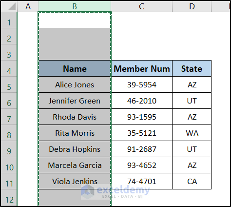
- Right-click on the column header before which you want to place the previous column.
- Select Insert Cut Cells from the context menu.
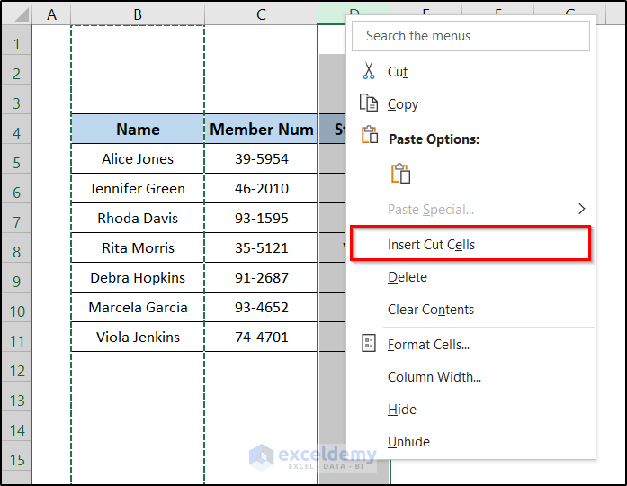
- This will insert the previous column there.
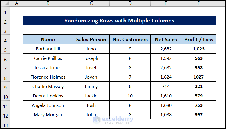
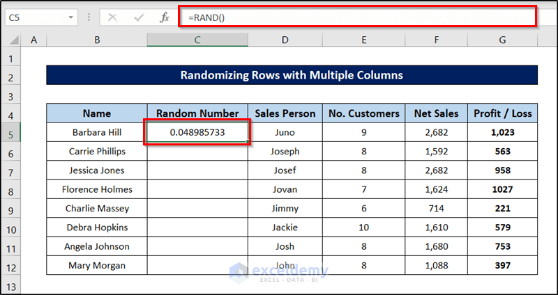
Method 11 – Randomize Rows
We’ll randomize the row order for the following dataset.
Steps:
- Click the header letter of column C, and the whole C column will be selected.
- Right-click and choose the Insert command, and a new column C will be created.
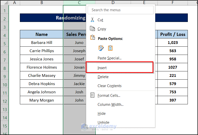
- Assign a name to the newly created column (i.e. Random Number).
- Select the first cell (i.e. C5) and insert the following formula into the cell.
=RAND()
- Press Enter, and a random number will be displayed in cell C5. The number is lower than 1.
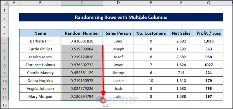
- Select the cell again and click and drag the fill handle icon to the end of the column to replicate the formula for the rest of the cells.
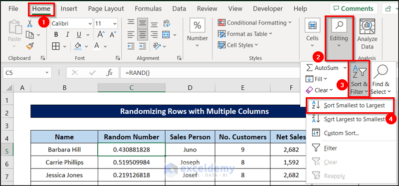
- With cell C5 selected, go to the Home tab.
- Go to the Editing group and click Sort & Filter.
- Select Sort Smallest to Largest from the drop-down menu.
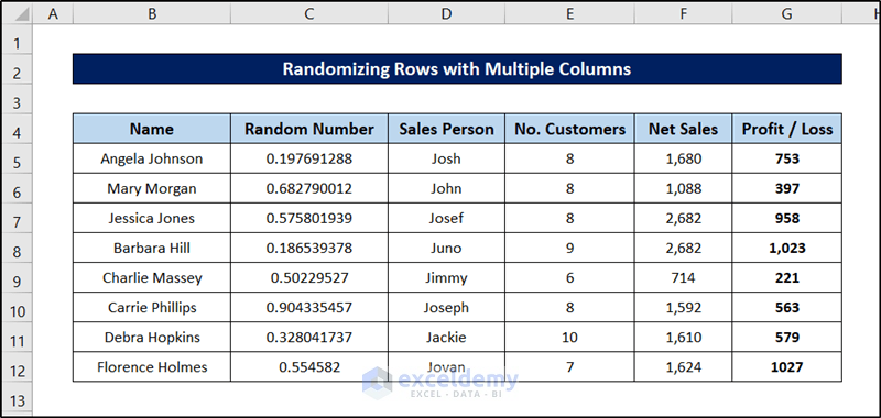
- The rows will randomize themselves. Excel will sort the dataset based on the values in column C, but the function in the column will then generate new values, so you can repeat the sort with different results.
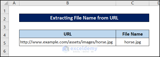
Method 12 – Extract the File Name from an URL
Steps:
- Cell B5 contains the URL of a file.
- Select the cell where you want to put the file name. In this case, it is cell C5.
- Use the following formula in it.
=RIGHT(B5,LEN(B5)-FIND("*",SUBSTITUTE(B5,"/","*",LEN(B5)-LEN(SUBSTITUTE(B5,"/","")))))
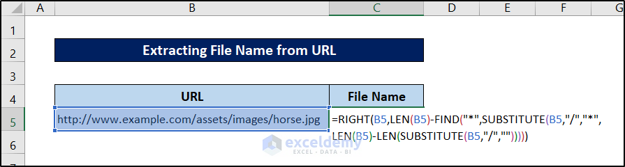
- Press Enter.
Breakdown of the Formula
SUBSTITUTE(B5,”/”,””) removes all the “/” from the URL. It returns http:www.example.comassetsimageshorse.jpg.
LEN(SUBSTITUTE(B5,”/”,””)) returns the length of the previous string.
LEN(B5) returns the length of the string in cell B4 which is 46 here.
LEN(B5)-LEN(SUBSTITUTE(B5,”/”,””))) indicates the difference between the two length values. This in turn indicates the number of “/” were removed.
SUBSTITUTE(B5,”/”,”*”,LEN(B5)-LEN(SUBSTITUTE(B5,”/”,””))) substitutes all the slashes (/) is cell B5 with star sign (*) with the instance number from the result of the previous function.
FIND(“*”,SUBSTITUTE(B5,”/”,”*”,LEN(B5)-LEN(SUBSTITUTE(B5,”/”,””)))) finds the position “*” is in the string up until now.
LEN(B5)-FIND(“*”,SUBSTITUTE(B5,”/”,”*”,LEN(B5)-LEN(SUBSTITUTE(B5,”/”,””)))) is the difference between the original string length and the previous position.
Finally, RIGHT(B5,LEN(B5)-FIND(“*”,SUBSTITUTE(B5,”/”,”*”,LEN(B5)-LEN(SUBSTITUTE(B5,”/”,””))))) extracts that number of characters from the right side of the cell.
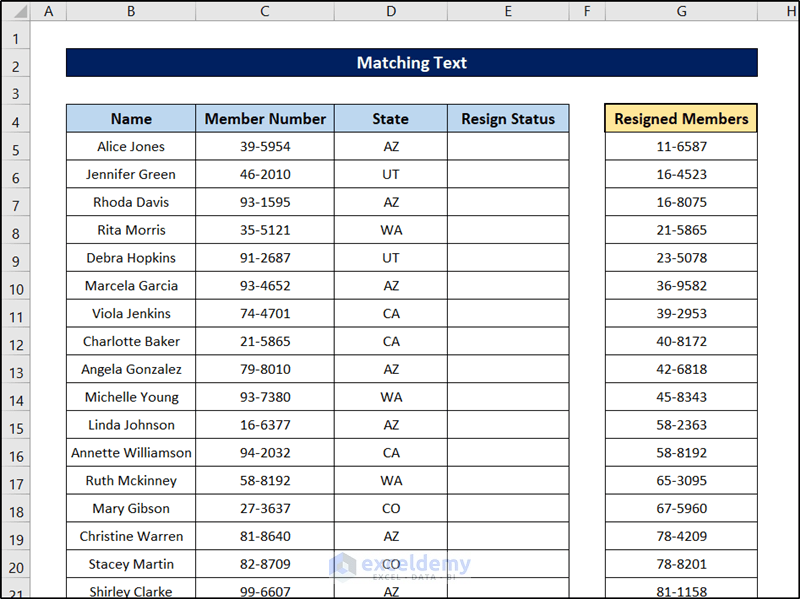
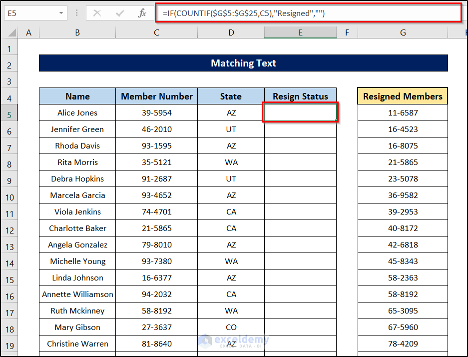
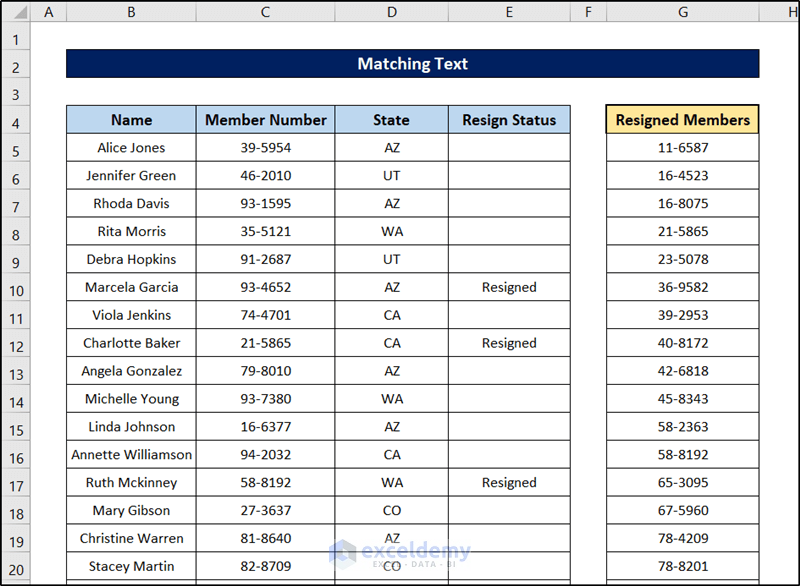
Method 13 – Match Text in List
We’ll find out the persons who have resigned from the left side of our example. There is a list on the right side of the resigned numbers. The data is in the range B5:D25.
Steps:
- Select cell E5.
- Insert the following formula.
=IF(COUNTIF($G$5:$G$25,C5),"Resigned","")
- Press Enter.
- Double-click the fill handle icon on the bottom-right corner of the cell border.
- The spreadsheet will look like this.
Read More: How to Remove Partial Data from Multiple Cells in Excel
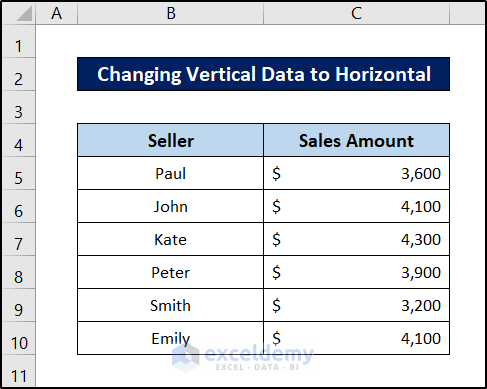
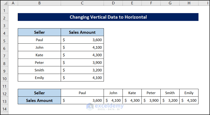
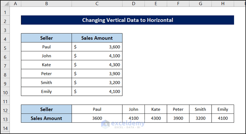
Method 14 – Change Vertical Data to Horizontal
We will be using the following dataset.
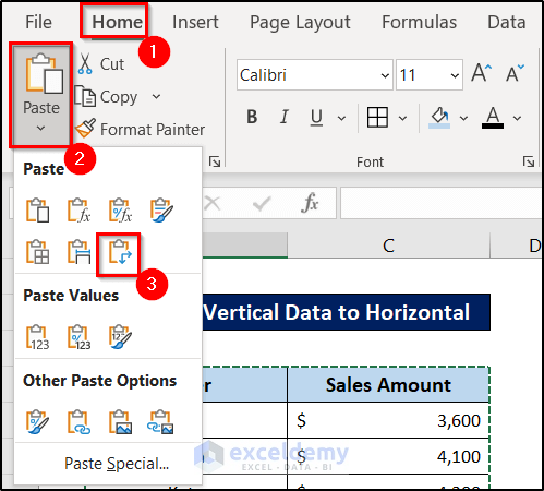
Using the Paste Special Option
- Select the range that you want to transpose. We have selected the range B4:C10.
- Press Ctrl + C to copy the range.
- Select a cell where you want to paste the range. We have selected cell B12.
- Select the Paste Transposed option from the Paste menu on the Home bar.
- This will change vertical columns into horizontal rows in the Excel spreadsheet.
Using the TRANSPOSE Function:
Steps:
- Select the cell where you want to place the formula.
- Use the following formula in it.
=TRANSPOSE(B4:C10)
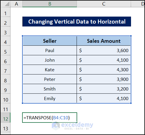
- Press Enter.
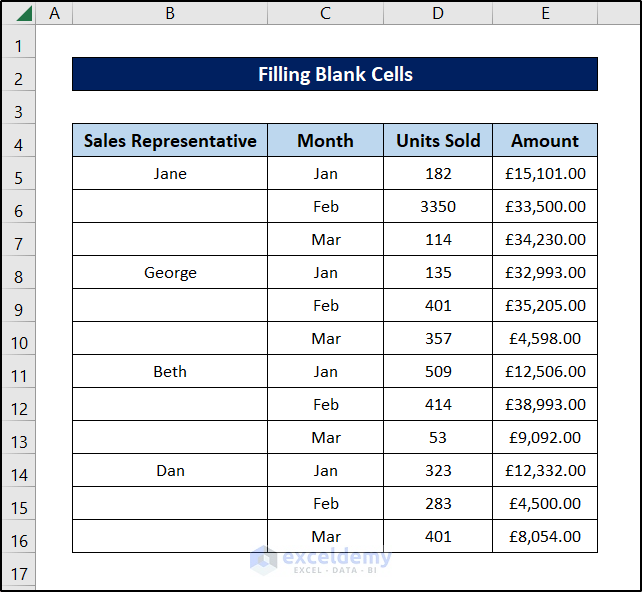
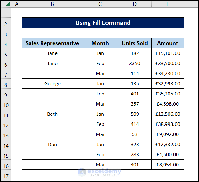
Method 15 – Fill Blank Cells
Here’s a sales dataset. We’ll fill the Sales Representative column by duplicating the entries from above.
Using the Fill Command
- Select cell B6.
- Go to the Home tab.
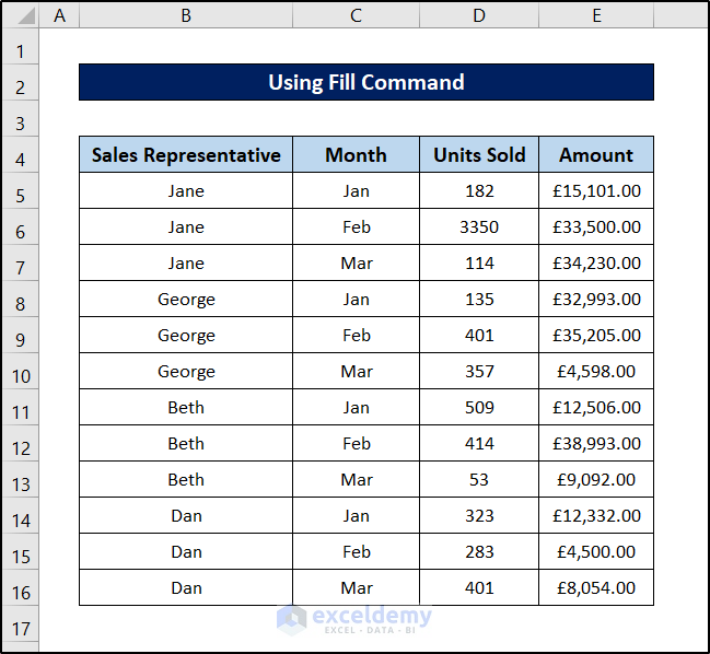
- From the Editing group, click on Fill and then Down.
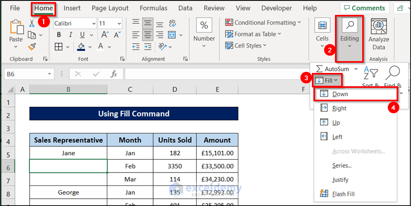
- The dataset will look like this now.
- Repeat the process for all the blank cells and fill out all the cells.
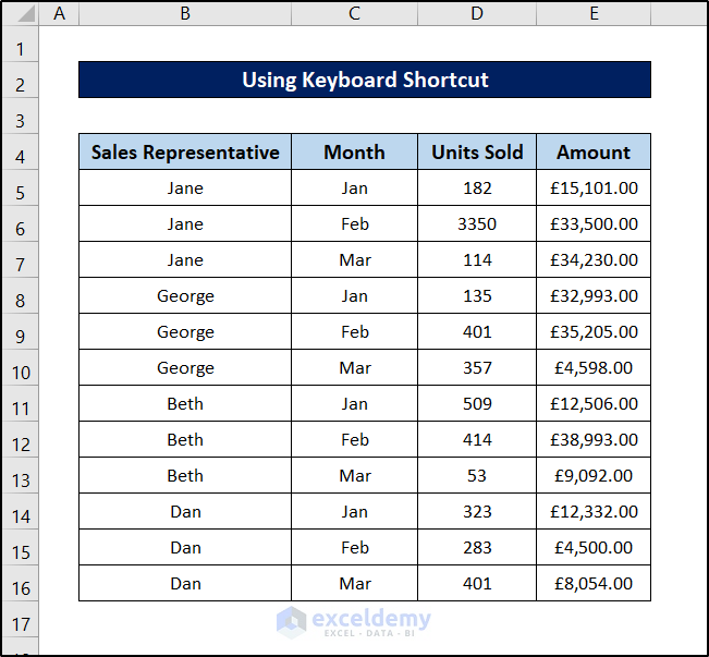
Using a Keyboard Shortcut:
- Select cell B6.
- Press Ctrl + D on your keyboard.
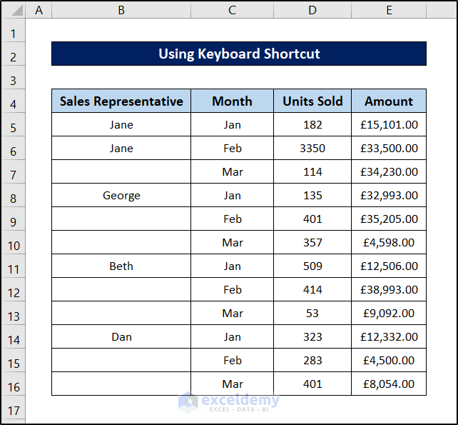
- Selecting cell B9 and pressing Ctrl + D will yield the following result.
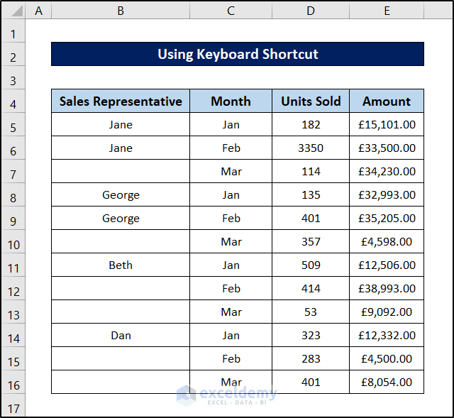
- Fill out all the blank values by selecting them and pressing the shortcut.
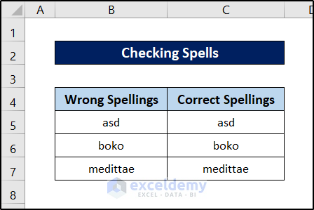
Method 16 – Check the Spelling
Here’s a sample dataset, where we’ll spellcheck column C.
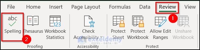
Steps:
- Select the range C5:C7.
- Go to the Review tab and select Spelling from the Proofing section. Alternatively, press F7 on your keyboard.
- Select the correct suggestion and click on Change to change the value of a particular cell. The errors come in the selection order here.
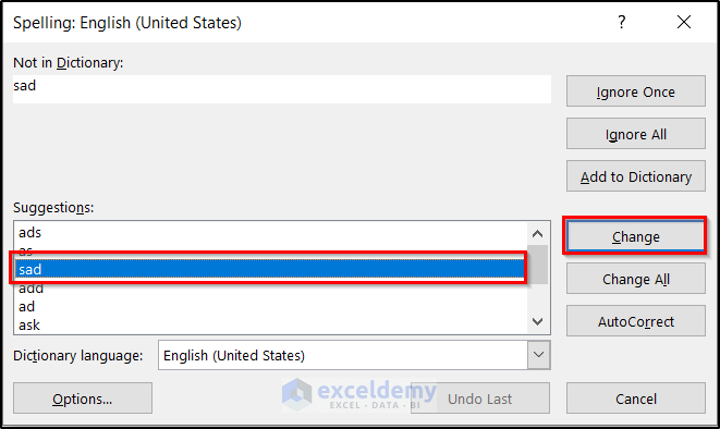
- This will change the first error in the dataset.
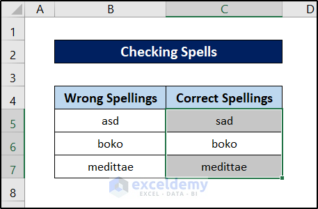
- Repeat this process for all the errors and you will have corrected spellings.

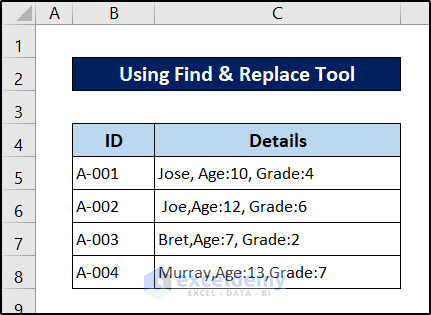
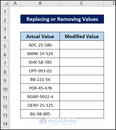
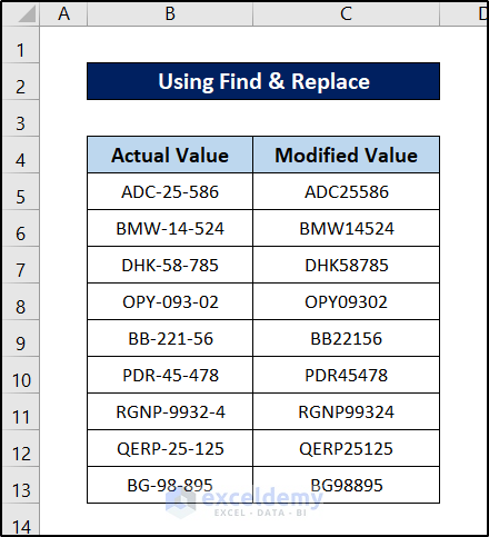
Method 17 – Replace or Remove Text
We have a sample dataset of IDs that we need to modify in some way.
Using the Find & Replace Feature:
- Select the range which you want to modify. In this case, it is C5:C13.
- Go to the Home tab.
- Select Find & Replace from the Editing section.
- Select Replace from the drop-down menu.
- Go to the Replace tab in the pop-up box.
- Insert the value you want to replace in the Find what field and the value you want to replace it with in the Replace with box.
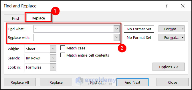
- Click Replace All to replace all of the values in the dataset.
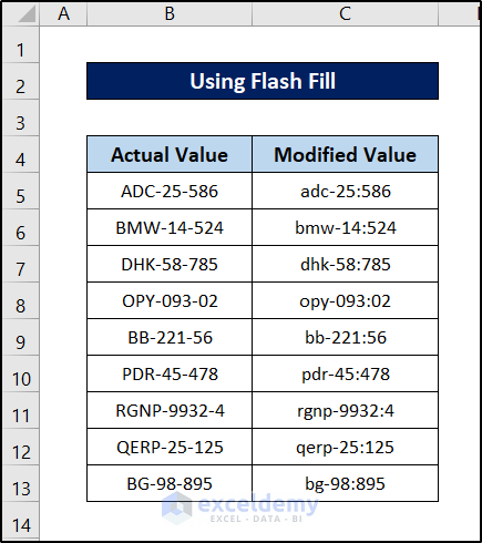
Utilizing Flash Fill:
- Write down the final product after removing or replacing the desired value in the first cell. We are replacing the second hyphen in the string with a colon.
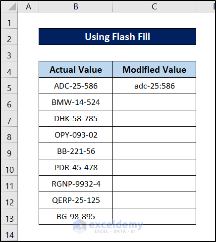
- Start writing the second one manually. As soon as you start writing, Excel will recognize the pattern and start suggesting the output for the rest.
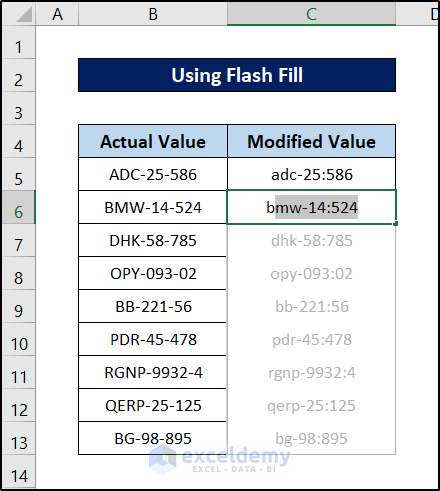
Note
Excel sometimes suggests the output at the third or fourth entry if the pattern isn’t that obvious.
- Press Enter.
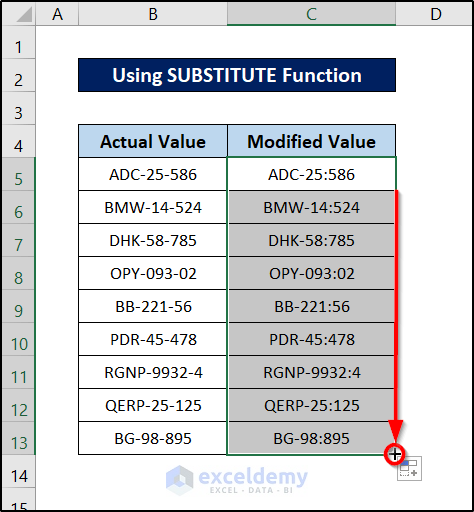
Using the SUBSTITUTE Function:
- Select cell C5.
- Use the following formula in it.
=SUBSTITUTE(B5,"-",":",2)
- Press Enter.
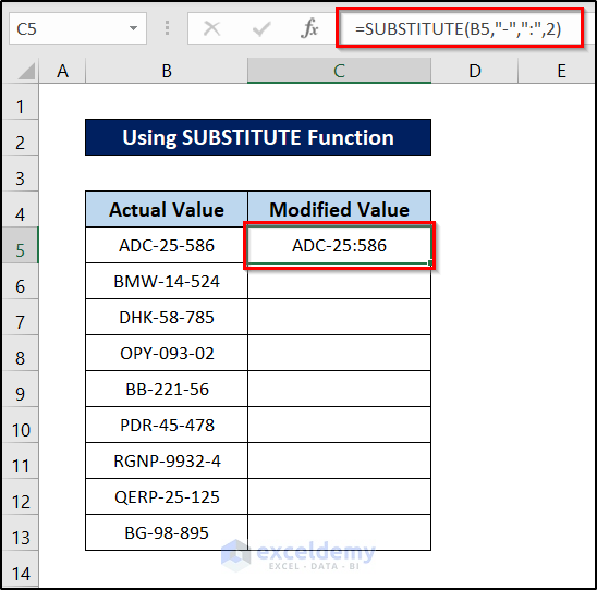
- Select the cell again and click and drag the fill handle icon to the end of the column to replicate the formula for the rest of the cells.
Read More: Using Excel to Clean and Prepare Data for Analysis
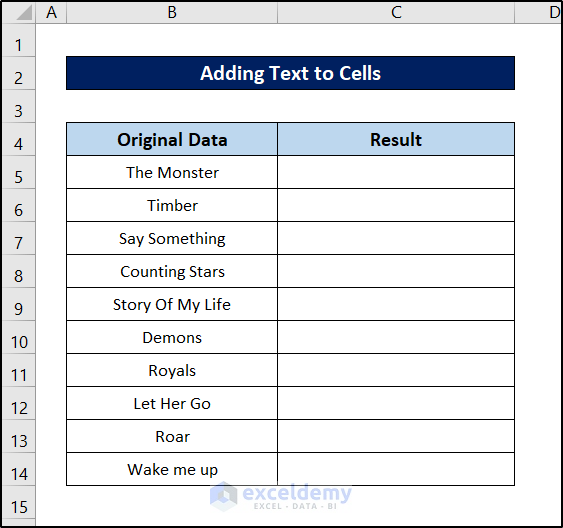
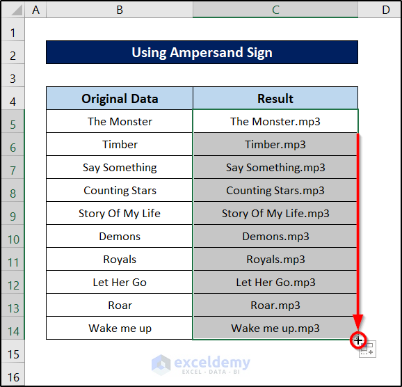
Method 18 – Add Text to Cells
Let’s add text at the end of the values in the following dataset.
Using the Ampersand (&) Symbol
- Select cell C5.
- Use the formula below.
=B5&".mp3"
- Press Enter.
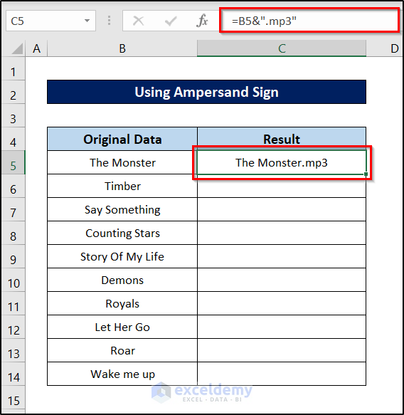
- Click and drag the fill handle icon to the end of the column to replicate the formula for the rest of the cells.
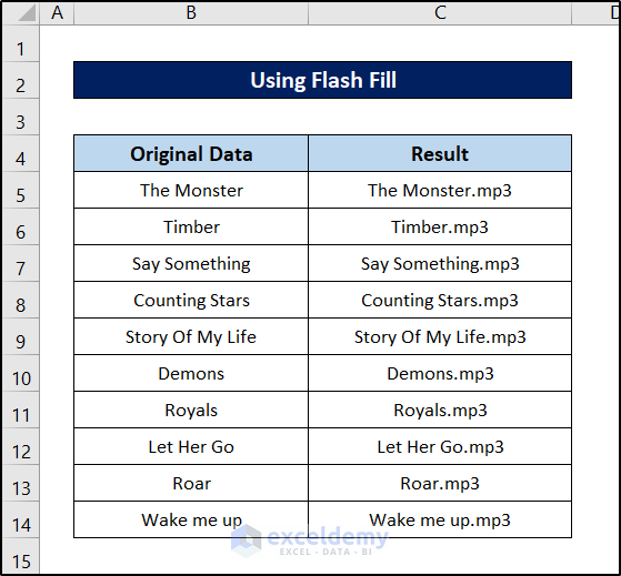
Applying the Flash Fill Feature:
- Write down the first intended value manually in cell C5.
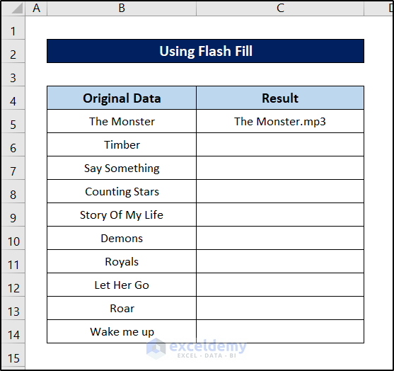
- Start filling out the second one in the dataset. Once you start filling, Excel will suggest the pattern.
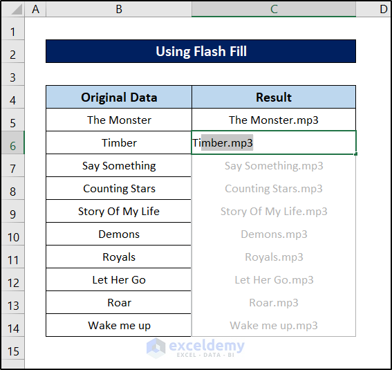
- As soon as the suggestion appears, press Enter.
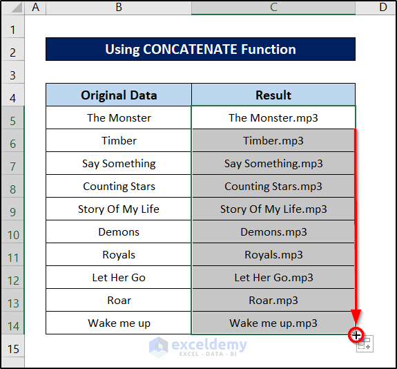
Using the CONCATENATE Function:
- Select cell C5.
- Use the following formula in it.
=CONCATENATE(B5,".mp3")
- Press Enter.
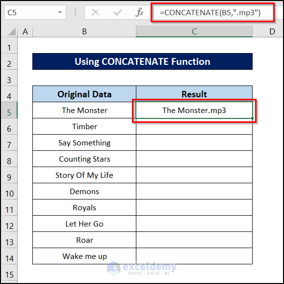
- Select the cell again and click and drag the fill handle icon to the end of the column to replicate the formula for the rest of the cells.
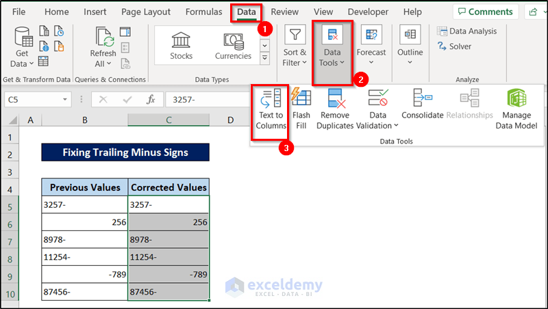
Method 19 – Fix Trailing Minus Sign
Sometimes while taking data from other sources, the negative values have a trailing minus sign. Here’s an example. Excel won’t recognize these as numbers, so we have to fix them.
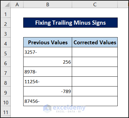
Steps:
- Select the range you want to convert. We have copied it to compare it with the previous one.
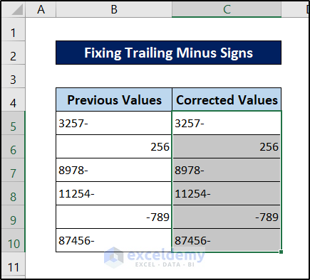
- Go to the Data tab on your ribbon.
- Select Text to Columns from the Data Tools group section.
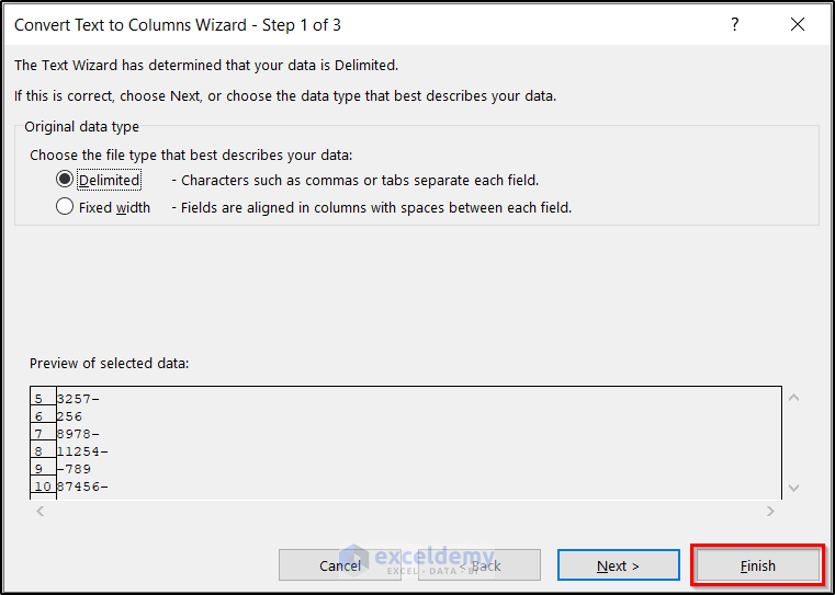
- Click on Finish in the wizard.
- This will automatically change all the negative values with trailing minus signs to Excel’s negative sign format.
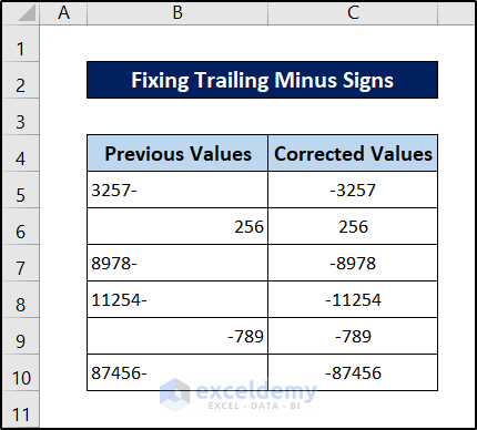
- This procedure works because there is a default setting in the Advanced Text Import Settings dialog box.
Download the Practice Workbook
Related Articles
<< Go Back To Data Cleaning in Excel | Learn Excel
Get FREE Advanced Excel Exercises with Solutions!

Super
Hello Satheesh,
Thanks for your appreciation. Glad to hear that you liked the article.
Keep exploring Excel with ExcelDemy!
Regards,
ExcelDemy