Looking for ways of using Excel to clean and prepare data for analysis? Then, this is the right place for you. Sometimes, the data we get is not clean and ready for analysis. In those cases, we need to clean and prepare data by following some steps. Here, you will find 10 different step-by-step explained ways to clean and prepare data for analysis using Excel.
10 Ways of Using Excel to Clean and Prepare Data for Analysis
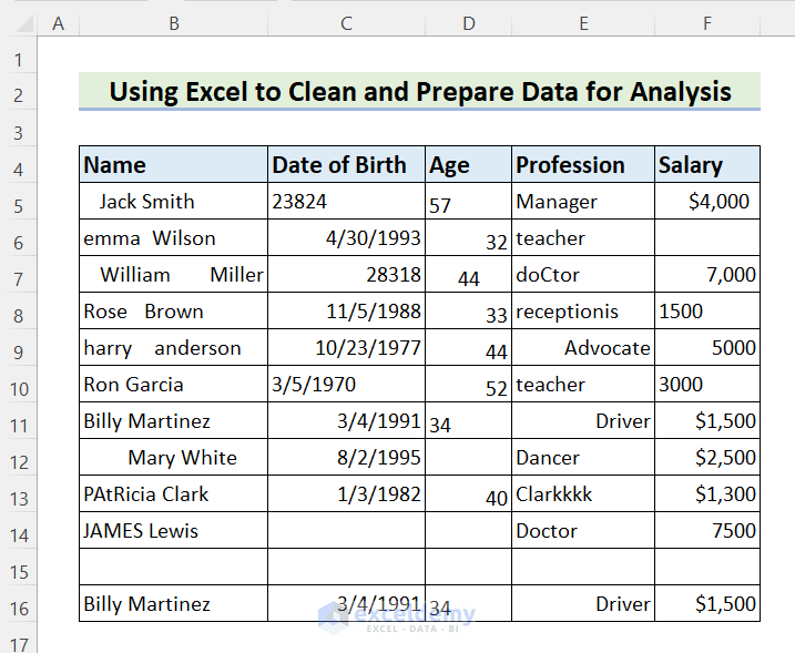
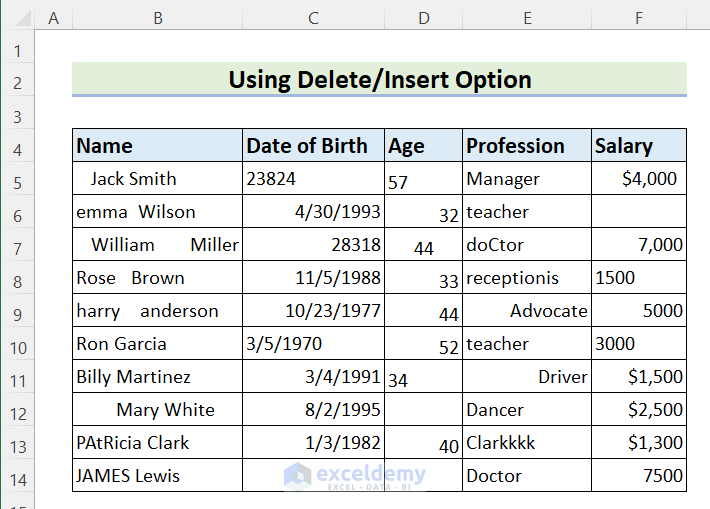
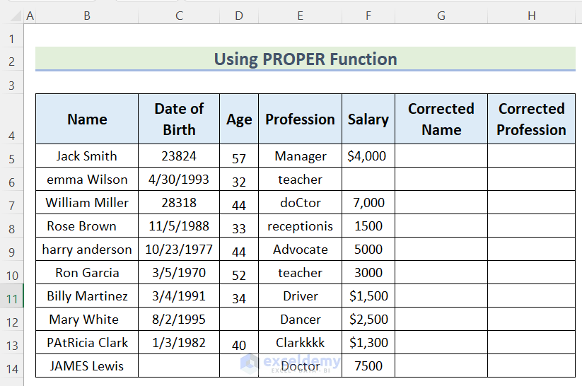
Here, we have a disorganized dataset containing Name, Date of Birth, Age, Profession and Salary of some people. Now, we will show you how to clean and prepare this dataset for analysis using Excel.
1. Using Remove Duplicates Feature to Clean and Prepare Data For Analysis
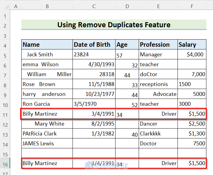
In the first method, we will remove the duplicate values by using the Remove Duplicates feature to clean and prepare data for analysis using Excel.
Steps:
- First, select Cell range B4:F16.
- Then, go to the Data tab >> click on Data Tools >> select Remove Duplicates.

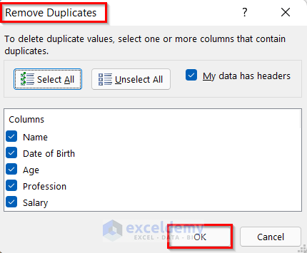
- Now, the Remove Duplicates dialog box will open.
- Then, press OK.
- After that, another box containing the information of the duplicates will appear.
- Next, press OK.

- Finally, the Remove Duplicates feature will remove the duplicate values from the dataset.

Read More: How to Clean Up Raw Data in Excel
2. Using Delete/Insert Option to Clean and Prepare Data in Excel
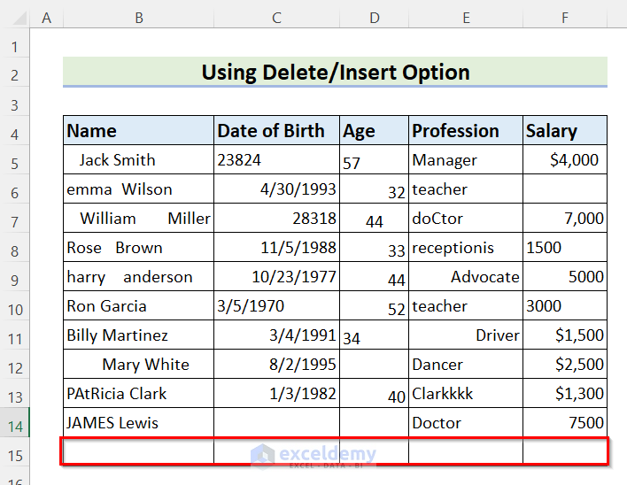
Next, we will use the Delete option to delete the blank row from the dataset to clean and prepare the data for analysis.
Steps:
- In the beginning, select Cell range B15:F15.
- Then, go to the Home tab >> click on Cells >> click on Delete >> select Delete Sheet Rows.

- Finally, the blank row will be deleted from the dataset using the Delete option.
Read More: How to Clean Survey Data in Excel
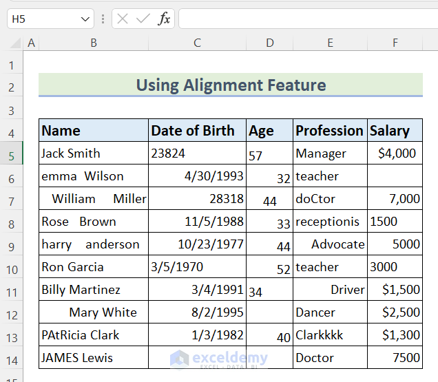
3. Using Alignment Feature to Clean and Prepare Data in Excel
In the third method, we will show you how to use the Alignment feature to clean and prepare data for analysis in Excel.
Follow the steps to do it on your own dataset.
Steps:
- First, select Cell range B4:F14.
- Then, go to the Home tab >> from Alignment Tools >> select Middle Align.

- Again, select Cell range B4:F14.
- Then, go to the Home tab >> from Alignment Tools >> select Center.

- Finally, the dataset is Middle and Center Aligned using the Alignment feature.

Read More: How to Do Automated Data Cleaning in Excel
4. Applying TRIM Function to Clean Data for Analysis in Excel
Now, we will show you how to trim the unwanted spaces in the dataset by applying the TRIM function to clean and prepare data for analysis in Excel.
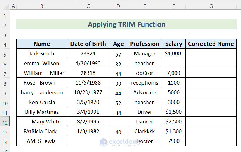
Steps:
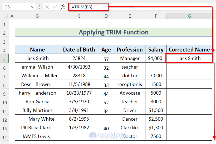
- First, select the Cell G5.
- Then insert the following formula.
=TRIM(B5)
Here, in the TRIM function, we selected Cell B5 as the text to trim the leading and trailing spaces of the selected cell.
- After that, press ENTER to get the value of Corrected Name.
- Then, drag down the Fill Handle tool to AutoFill the formula for the rest of the cells.
- Finally, the TRIM function has removed the unwanted spaces from column B.

5. Using PROPER Function to Clean and Prepare Data in Excel
Next, we will change the text case using the PROPER function to clean and prepare data for analysis in Excel.
Steps:
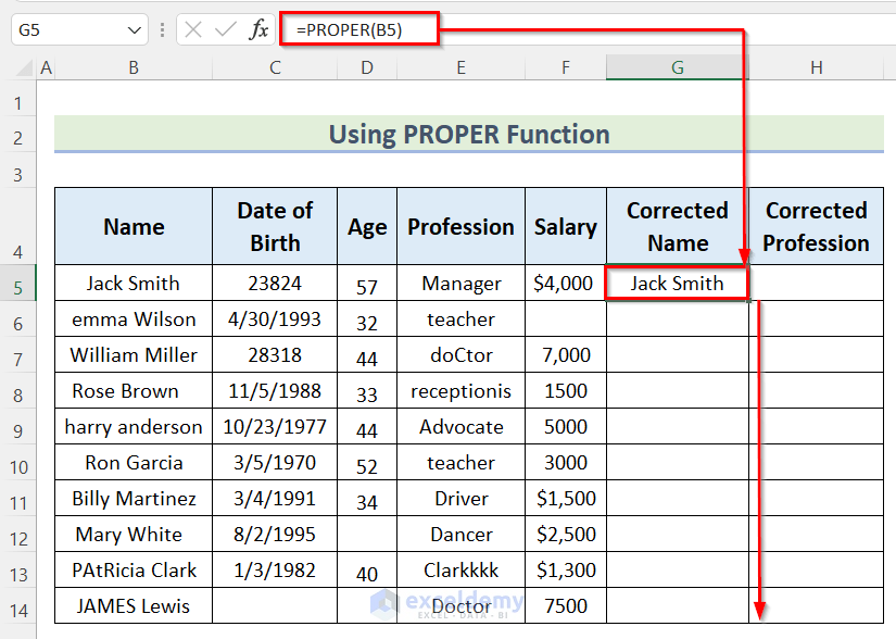
- First, select the Cell G5.
- Then insert the following formula.
=PROPER(B5)
Here, in the PROPER function, we selected Cell B5 to change the first lower case to upper case and middle-upper cases to lower case cell. Finally, it will return the proper format of texts.
- After that, press ENTER to get the value of Corrected Name.
- Then, drag down the Fill Handle tool to AutoFill the formula for the rest of the cells.
- Now, you will get the values of the Corrected Name.

- After that, select the Cell H5.
- Then insert the following formula.
=PROPER(E5)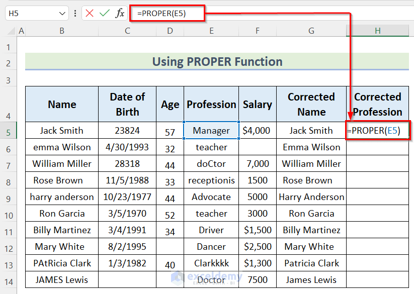
Here, in the PROPER function, we selected Cell E5 as the text to trim the cell.
- After that, press ENTER to get the value of Corrected Profession.
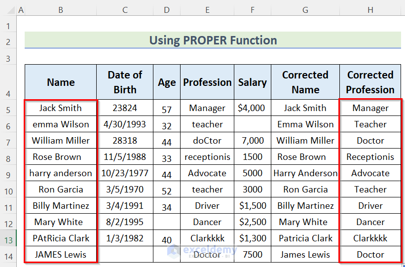
- Then, drag down the Fill Handle tool to AutoFill the formula for the rest of the cells.

- Finally, you will get the values of Corrected Profession.
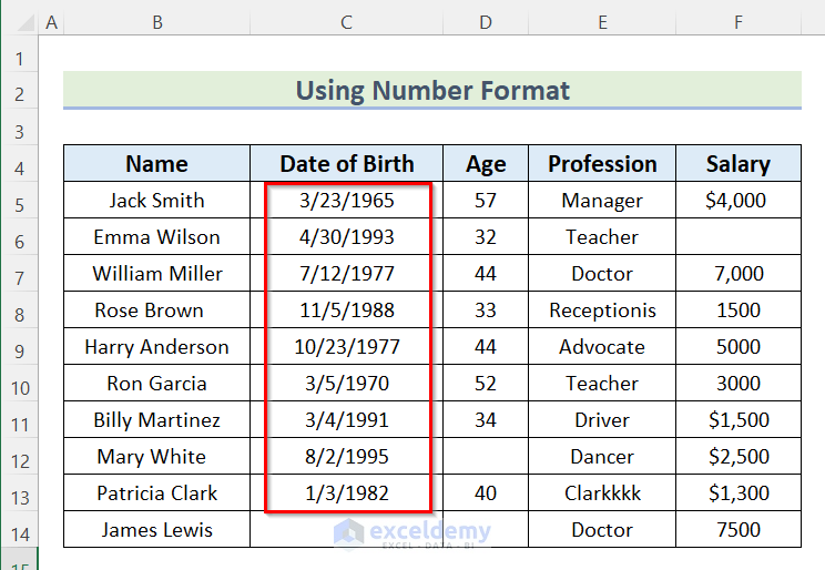
6. Using Number Format to Prepare Data for Analysis
Now, we will use the Number format in column C and column F to clean and prepare data for analysis in Excel.

Steps:
- First, select Cell range C5:C14.
- Then, go to the Home tab >> click on Number >> select Short Date.

- Now, you will find all the values of the Date of Birth in the same format.
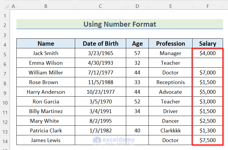
- First, select Cell range F5:F14.
- Then, go to the Home tab >> click on Number >> select Currency.

- Finally, you will find all the values of Salary in Currency format.
7. Using Spell Check to Clean Data for Analysis in Excel
Now, we will check the spelling of the values of the dataset and change incorrect spellings using Spell Check in Excel to clean and prepare data for analysis.
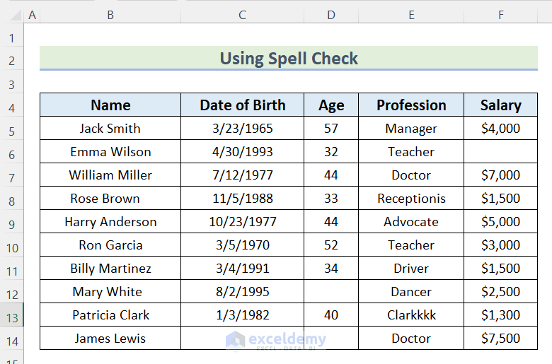
Steps:
- First, select Cell range B4:F14.
- Then, go to the Review tab and click on Spelling.

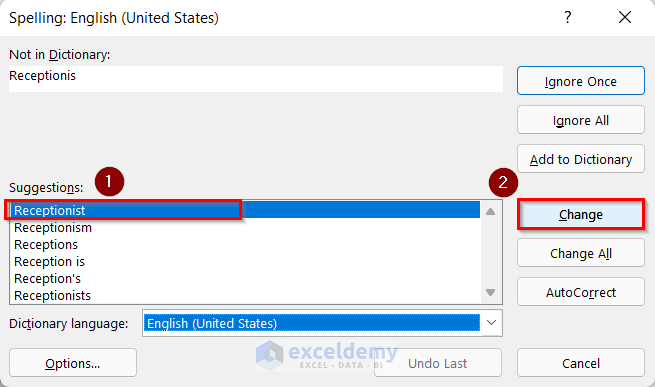
- After that, the Spelling dialog box will open.
- Now, select the spelling “Receptionist”.
- Then, click on Change.
- Next, select the spelling “Clerk”.
- Then, click on Change.

- After that, a box will open to confirm the spell check.
- Now, press OK.
- Finally, the spelling mistakes are corrected using Spell Check.

Read More: 19 Practical Data Cleaning Techniques in Excel
8. Use of Conditional Formatting to Detect Blank Cells in Excel
Now, we will use Conditional Formatting to detect blank cells to clean and prepare data for analysis in Excel.
Steps:
- First, select Cell range B4:F14.
- Then, go to the Home tab >> click on Conditional Formatting.
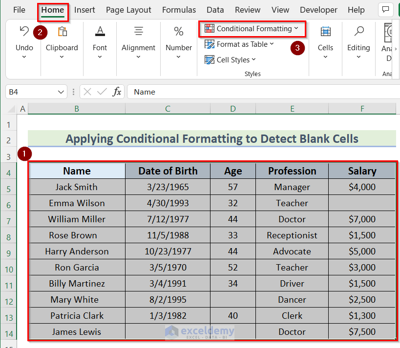
- After that, select New Rules.

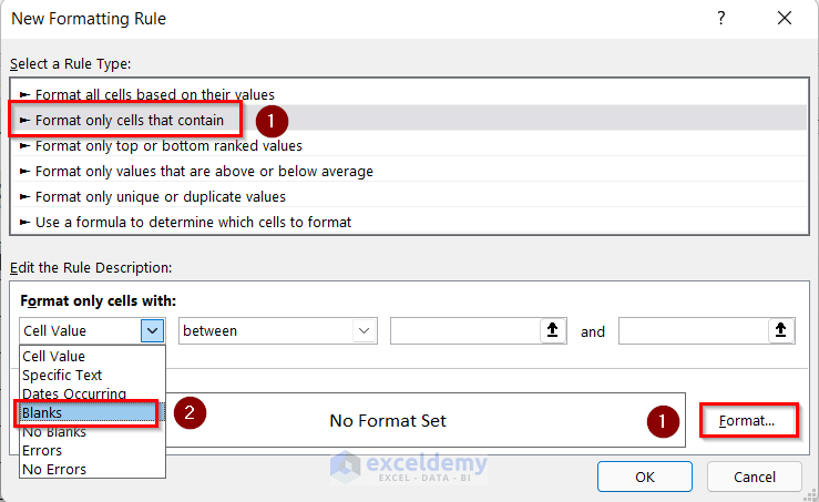
- Then, New Formatting Rule dialog box will appear.
- Now, select Format only cells that contain.
- After that, Blanks as Format only cells with.
- Then, click on the Format button.
- Now, the Format Cells dialog box will open.
- Then, go to the Fill section.
- Next, select a color of your own choice. Here, we will choose red.
- After that, press OK.

- Finally, press OK.
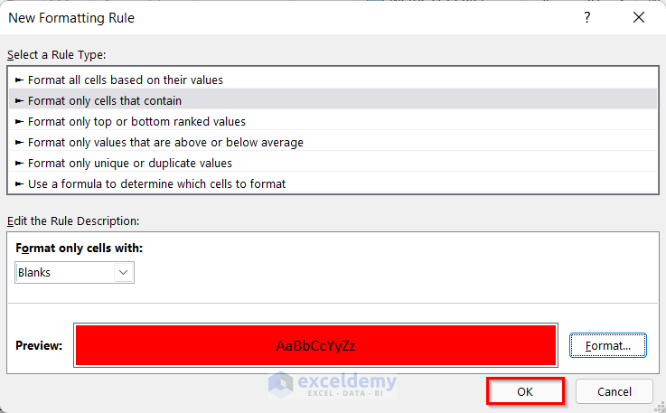
- Thus, you can detect the black cells in excel using Conditional Formatting.

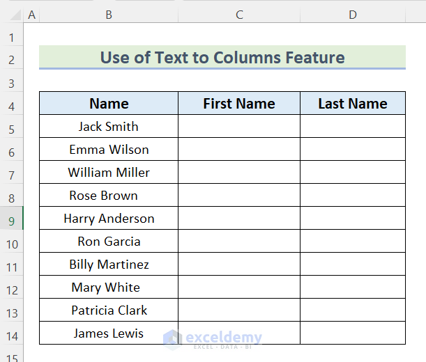
9. Use of Text to Columns Feature to Clean and Prepare Data
Here, in the dataset, we have both the first and last name of a person in the same column titled as Name. We can separate the data into two different columns using the Text to Columns feature to clean and prepare data for analysis in Excel.
Steps:
- In the beginning, select Cell range B5:B14
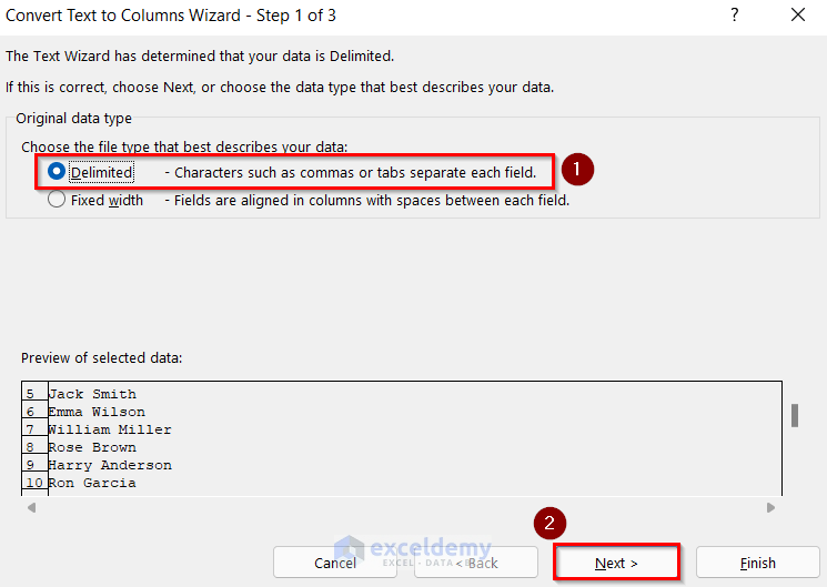
- Then, go to the Data tab >> click on Data Tools >> select Text to Columns.

- Next, select Delimited.
- Then, click on Next.
- After that, select Space as Delimiters.
- Then, click on Next.

- Next, insert Cell C5 as Destination.
- Now, click on Finish.
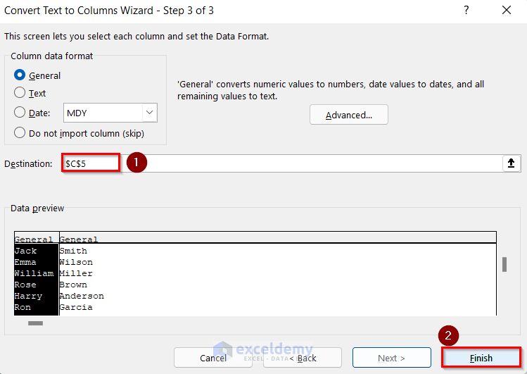
- Finally, you can see that the data have been divided into two columns First Name and Last Name.

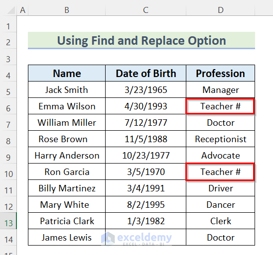
10. Using Find and Replace Option to Clean and Prepare Data
In the final method, we will clean and prepare the dataset for analysis using the Find and Replace option in Excel. Here, we can see two values containing “#”. We will replace this value with blank by applying Find and Replace option.
Steps:
- First, select Cell range B4:D14.
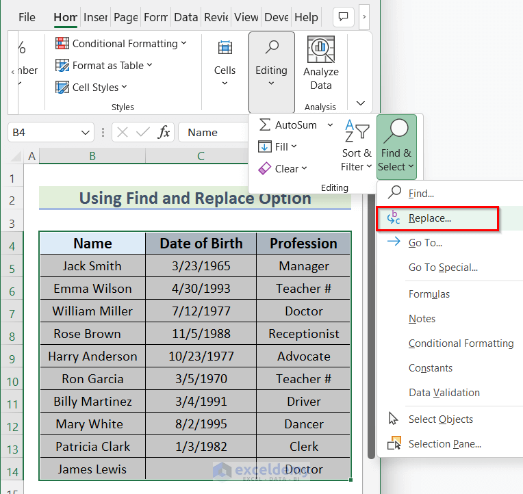
- Then, go to the Home tab >> click on Editing >> click on Find & Select.

- Next, select Replace.
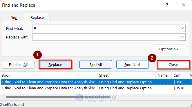
- Now, the Find and Replace toolbox will open.
- Then, insert “#” in the Find what box and blank in the Replace with box.
- After that, click on Find All.

- Next, click on Replace.
- Then, click on Close.
- Finally, the dataset has been cleared and prepared using the Find and Replace option in Excel.

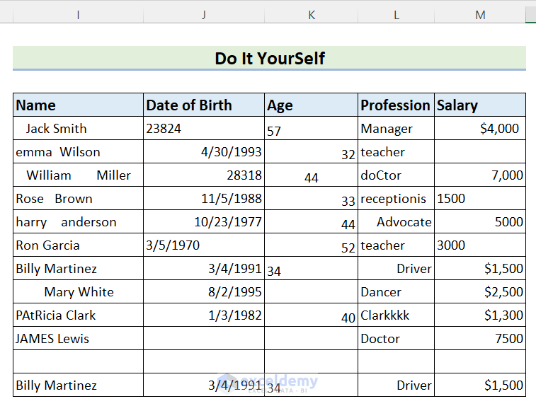
Practice Section
In the article, you will find an Excel workbook like the image given below to practice on your own.
Download Practice Workbook
Conclusion
So, in this article, we have shown you ways of using Excel to clean and prepare data for analysis. I hope you found this article interesting and helpful. If something seems difficult to understand, please leave a comment. Please let us know if there are any more alternatives that we may have missed. Thank you!
Related Articles
<< Go Back To Data Cleaning in Excel | Learn Excel
Get FREE Advanced Excel Exercises with Solutions!
