How to Remove Numbers from a Cell in Excel (7 Effective Ways)

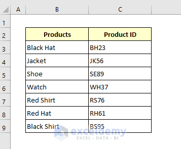
We have placed some Product Names and their IDs in the dataset. We want to remove the numbers from the Product IDs.

Method 1 – Using Find & Replace with Wildcards to Remove Numbers from a Cell in Excel

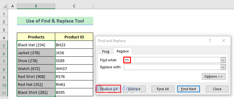
We have some numbers in parentheses in the Products Names column. We will remove these numbers.

Steps:

• Select the data range B5:B11.
• Press Ctrl + H to open Find & Replace command.
• Type (*) in the Find what box and keep the Replace with box empty.
• Press Replace All.

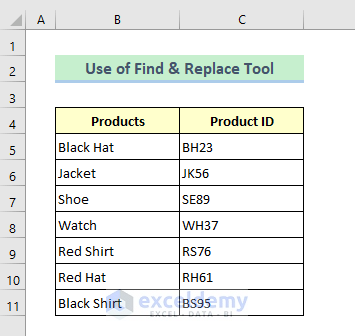
• Close the dialog to see the results.

Read More: How to Remove Value in Excel

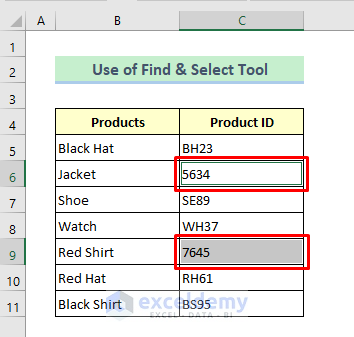
Method 2 – Applying the Find & Select Tool to Delete Numbers from a Cell

There are two cells in the Product IDs column which contain numbers only. We’ll remove the numbers from the ID cells.

Steps:

• Select the data range C5:C11.
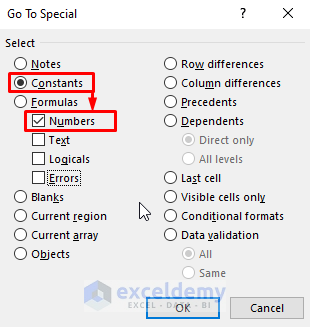
• Go to the Home tab, select Find & Select, and choose Go to Special
• A dialog box will open up.

• Mark only Numbers from the Constants options.
• Press OK.

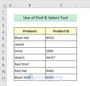
• Only the numbers are highlighted.

• Press the Delete button on your keyboard.

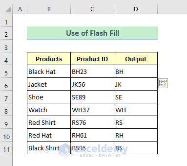
Method 3 – Using Flash Fill to Remove Numbers from a Cell in Excel

Steps:

• Type only the text (not the digits) of the first cell to a new column adjacent to it.
• Hit the Enter button.

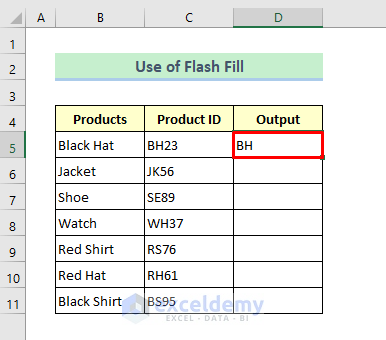
• Select Cell D5.
• Go to Data, then to Data Tools, and select Flash Fill.

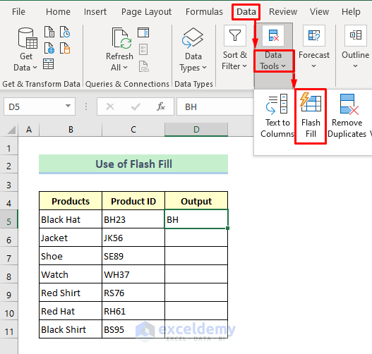
• The numbers are removed.

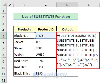
Method 4 – Inserting the SUBSTITUTE Function to Remove Numbers from a Cell in Excel

Steps:

• Use the formula given below in Cell D5:

• Hit Enter.

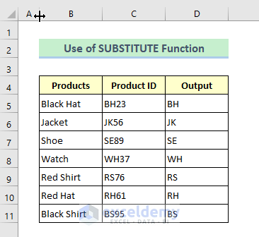
• Double-click the Fill Handle icon, and the formula will be copied down automatically.

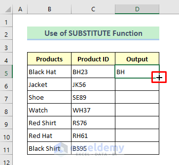
• The numbers are removed from the cells.

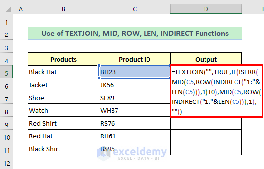
Method 5 – Combine TEXTJOIN, MID, ROW, LEN, and INDIRECT Functions to Delete Numbers

Steps:

• Use this formula in Cell D5:

• Hit the Enter button.

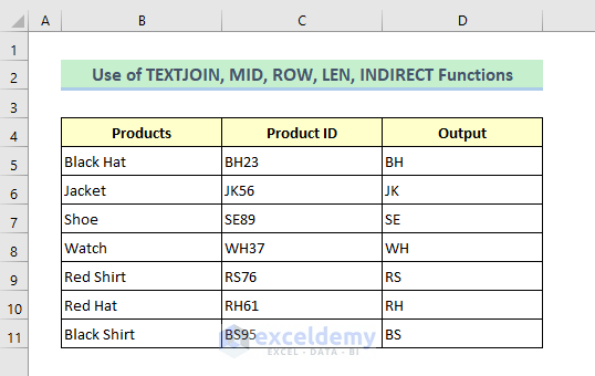
• Drag the Fill Handle icon down to copy the formula.

Formula Breakdown:

➥ ROW(INDIRECT(“1:”&LEN(C5)))

It will find the resultant array list from the ROW and INDIRECT functions that returns as-

{1;2;3;4}

➥ MID(B3,ROW(INDIRECT(“1:”&LEN(B3))),1)

The MID function is applied to extract the alphanumeric string based on the start_num and num_chars arguments.And for the num-chars argument, we’ll put 1. After putting the arguments in the MID function, it will return an array like-

{“B”;”H”;”2″;”3″}

➥ ISERR(MID(B3,ROW(INDIRECT(“1:”&LEN(B3))),1)+0)

After adding 0, the output array is put into the ISERR function. It’ll create an array of TRUE and FALSE, TRUE for non-numeric characters, and FALSE for numbers. The output will return as-

{TRUE;TRUE;FALSE;FALSE}

➥ IF(ISERR(MID(B3,ROW(INDIRECT(“1:”&LEN(B3))),1)+0),MID(B3,ROW(INDIRECT(“1:”&LEN(B3))),1),””)

The IF function will check the output of the ISERR function. If its value returns TRUE, it will return an array of all the characters of an alphanumeric string. So we have added another MID function. If the value of the IF function is FALSE, it will return blank (“”). So finally we’ll get an array that contains only the non-numeric characters of the string. That is-

{“B”;”H”;””;””}

➥ TEXTJOIN(“”,TRUE,IF(ISERR(MID(B3,ROW(INDIRECT(“1:”&LEN(B3))),1)+0),MID(B3,ROW(INDIRECT(“1:”&LEN(B3))),1),””))

The TEXTJOIN function will join all the characters of the above array and avoid the empty string. The delimiter for this function is set as an empty string (“”) and the ignored empty argument’s value is entered TRUE. This will give our expected result-

{BH}

Read More: How to Remove Outliers in Excel

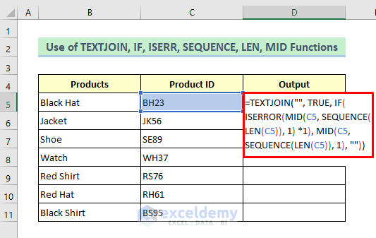
Method 6 – Apply TEXTJOIN, IF, ISERROR, SEQUENCE, LEN, and MID Functions to Remove Numbers

Steps:

• In Cell D5, insert the following formula:

• Press the Enter button to get the result.

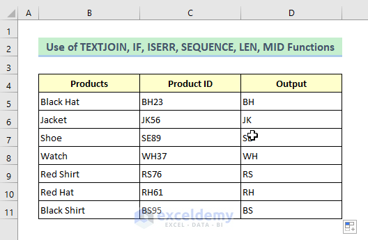
• Apply the AutoFill option to copy the formula.

Formula Breakdown:

➥ LEN(C5)

The LEN function will find the string length of Cell C5 that will return as-

{4}

➥ SEQUENCE(LEN(C5))

Then the SEQUENCE function will give the sequential number according to the length that returns as-

{1;2;3;4}

➥ MID(C5, SEQUENCE(LEN(C5)), 1)

The MID function will return the value of that previous position numbers which results-

{“B”;”H”;”2″;”3″}

➥ ISERROR(MID(C5, SEQUENCE(LEN(C5)), 1) *1)

Now the ISERROR function will show TRUE if it finds an error otherwise it will show FALSE. The result is-

{TRUE;TRUE;FALSE;FALSE}

➥ IF(ISERROR(MID(C5, SEQUENCE(LEN(C5)), 1) *1), MID(C5, SEQUENCE(LEN(C5)), 1), “”)

Then the IF function sees TRUE, it inserts the corresponding text character into the processed array with the help of another MID function. And sees FALSE, it replaces it with an empty string:

{“B”;”H”;””;””}

➥ TEXTJOIN(“”, TRUE, IF(ISERROR(MID(C5, SEQUENCE(LEN(C5)), 1) *1), MID(C5, SEQUENCE(LEN(C5)), 1), “”))

The final array will be passed over to the TEXTJOIN function, so it concatenates the text characters and outputs the result as-

{BH}

Method 7 – Removing Numbers from a Cell with a User-defined Function in Excel VBA 

Case 1 – Remove Numbers from a Cell

Steps:

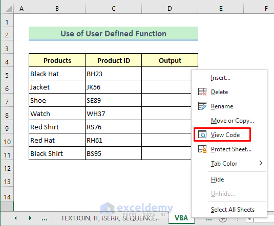
• Right-click on the sheet title.
• Select View Code from the context menu.
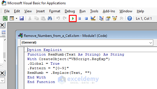
• A VBA window will appear.

• Insert the following code in the window:

Option Explicit
Function RemNumb(Text As String) As String
With CreateObject("VBScript.RegExp")
.Global = True
.Pattern = "[0-9]"
RemNumb = .Replace(Text, "")
End With
End Function

• Press the Play icon to run the macro.

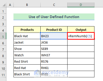
• In Cell D5, insert:

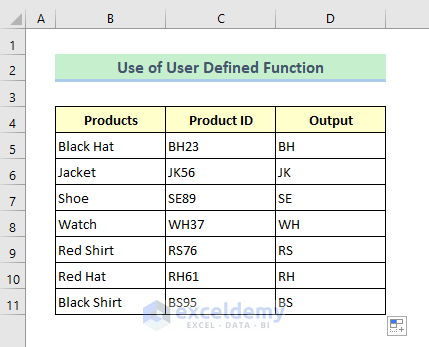
• Hit the Enter button to get the result.

• Drag the Fill Handle icon to copy the formula.

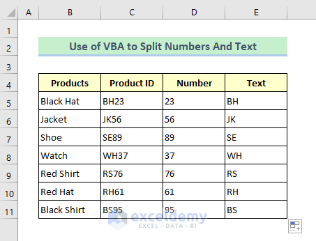
Case 2 – Split Numbers and Text into Separate Columns

Steps:

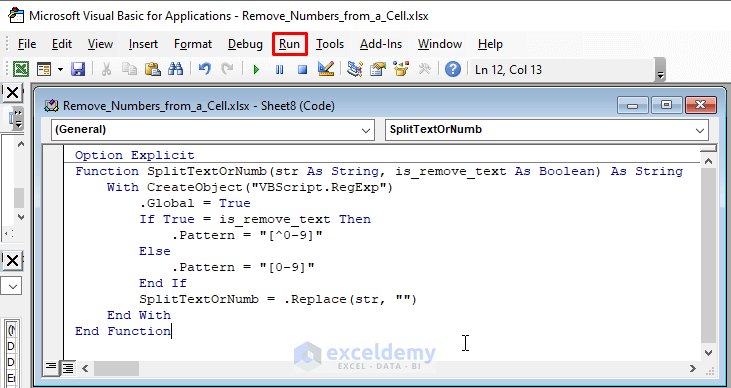
• Open the VBA window and insert the following code:

Option Explicit
Function SplitTextOrNumb(str As String, is_remove_text As Boolean) As String
    With CreateObject("VBScript.RegExp")
        .Global = True
        If True = is_remove_text Then
            .Pattern = "[^0-9]"
        Else
            .Pattern = "[0-9]"
        End If
        SplitTextOrNumb = .Replace(str, "")
    End With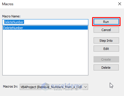
End Function

• Click Run and a Macro will open up.

• Select the macro and press Run.

• Insert the following formula in Cell D5:

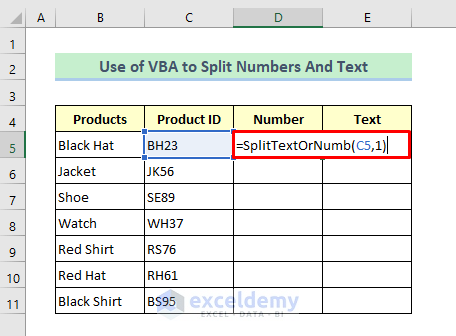
• To delete numeric characters:

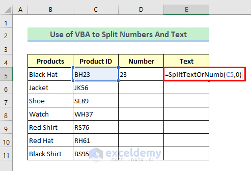
• Press the Enter button and use the Fill Handle tool to copy the formula.

Download the Practice Workbook

Related Articles

• How to Remove Compatibility Mode in Excel
• How to Remove 0 from Excel
• How to Remove Drop Down Arrow in Excel
• How to Remove HTML Tags from Text in Excel

<< Go Back To Data Cleaning in Excel | Learn Excel