Panes allow you to freeze one portion of your Excel datasheet and scroll the other portion separately. Though it is a useful feature, you may need to remove panes in different situations. The earlier article might help you to add panes, following the continuity, in this article, I’ll show you how to remove panes in Excel in 4 different ways.
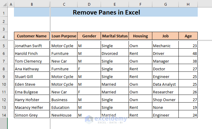
Suppose, you have the following dataset with panes. Now, go through the rest of the article to know the ways of removing panes in Excel.
4 Ways to Remove Panes in Excel
1. Remove Panes With Double Click
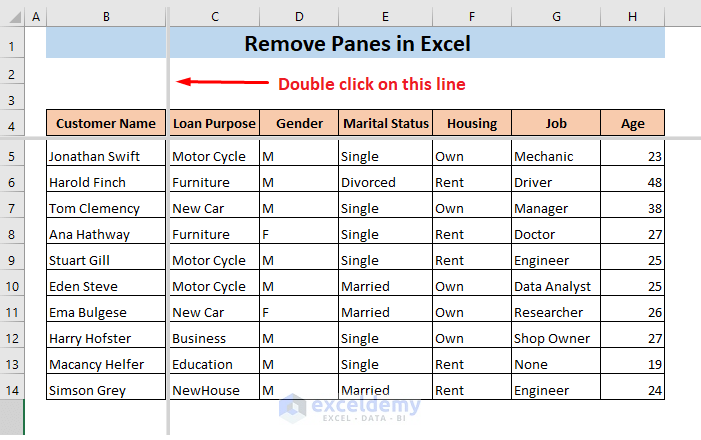
The easiest way to remove panes is to double click on the panes.
➤ Keep your cursor on one of the panes and double click on it.
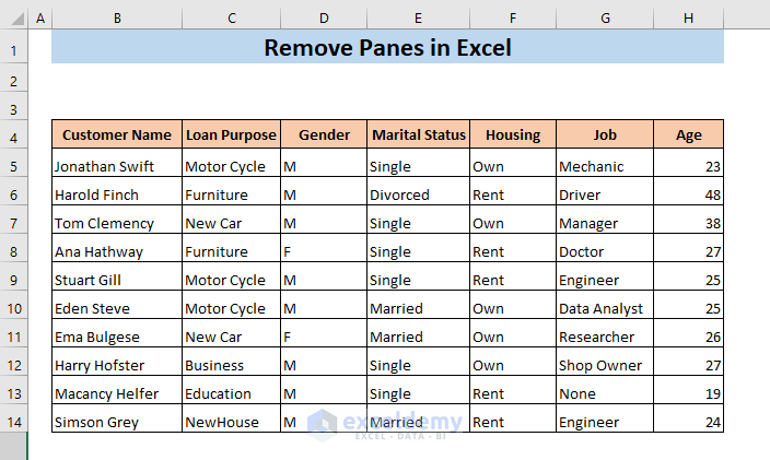
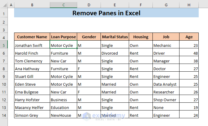
As a result, this pane will be removed.
In a similar way click on the other pane to remove it.
Read More: How to Remove Value in Excel
2. Remove Panes Using Split from View Tab
You can also remove panes from the view tab.
➤ Go to the View tab and select the Split icon from the Window tab.
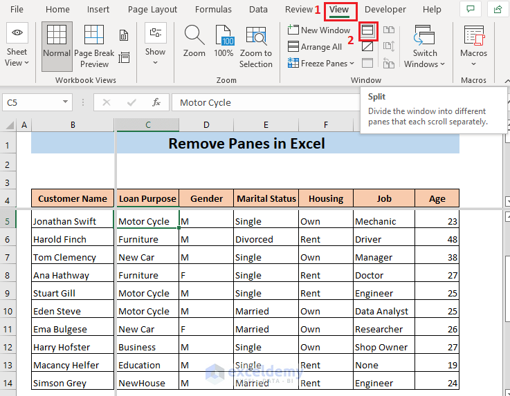
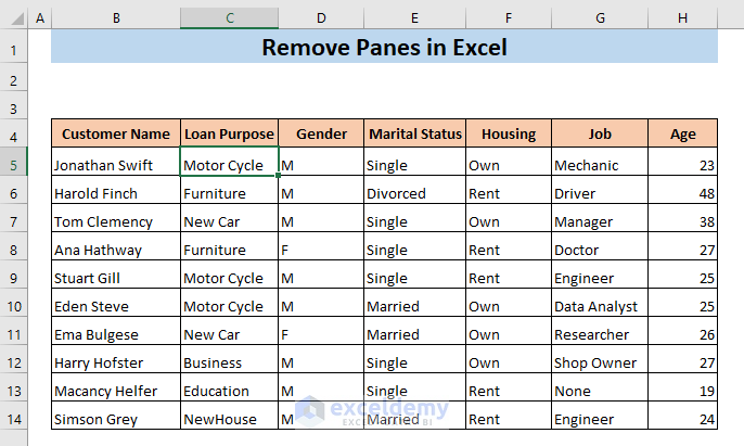
As a result, the panes will be removed from your Excel datasheet.

Read More: How to Remove Dotted Lines in Excel
3. Keyboard Shortcut Key to Remove Panes
In this section, I’m going to share with you a way that you may find easy to use if you like the keyboard rather than the mouse. Let’s how to use a keyboard shortcut key to remove panes.
➤ To remove panes, press,
ALT+W+S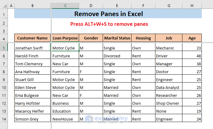
It will remove all the panes from your Excel worksheet.
4. Unfreeze Panes
If you activate the panes from the Freeze Panes option, you can remove them with the Unfreeze Panes option.
➤ Go to View > Freeze Panes and select Unfreeze Panes.
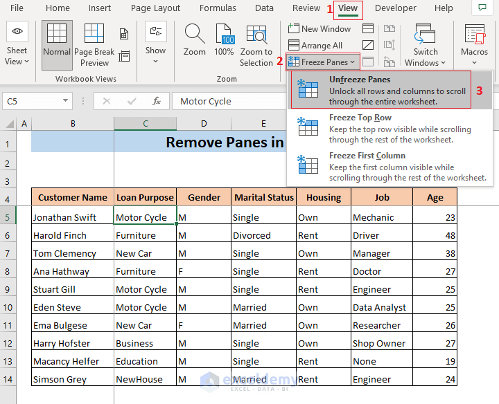
It will remove all the panes from your Excel worksheet.
Read More: How to Remove Outliers in Excel
Practice Section
I have added a dedicated worksheet named “Practice” in the Excel file. You can download the workbook from the Download Practice Workbook section and practice removing panes from the “Practice” worksheet.
Download Practice Workbook
Conclusion
I hope now you know how to remove panes in Excel. If you have any confusion feel free to leave a comment.
Related Articles
- How to Remove Numbers from a Cell in Excel
- How to Remove Compatibility Mode in Excel
- How to Remove Drop Down Arrow in Excel
- How to Remove HTML Tags from Text in Excel
- How to Remove 0 from Excel
<< Go Back To Data Cleaning in Excel | Learn Excel
Get FREE Advanced Excel Exercises with Solutions!
