Here’s an overview of how you can ignore the N/A values or errors in a SUM function. The following picture shows all the formulas we’ll use.
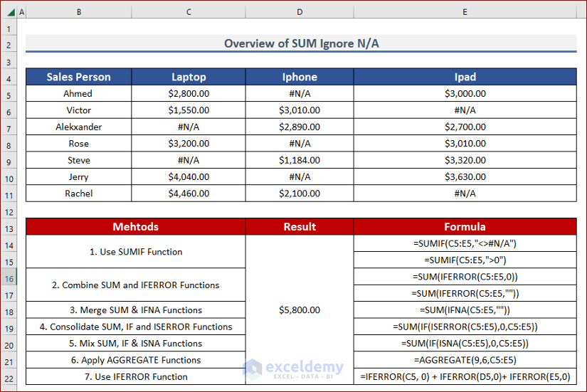
7 Simple Ways to SUM While Ignoring N/A in Excel
Our sample dataset contains three columns (C through E) of items sold, but not all cells in the columns contain a value. We’ll sum these columns row-wise and display the result in column F.
Method 1 – Use the SUMIF Function to SUM and Ignore N/A Errors
Steps:
- Select the result cell, such as E5.
- Insert the following formula and press Enter.
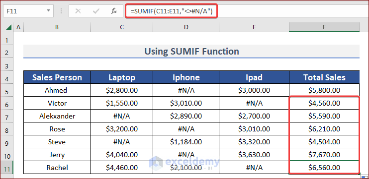
=SUMIF(C5:E5,"<>#N/A")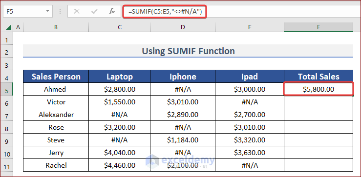
- Use the Fill Handle to AutoFill formula for the rest of the cells in the column.
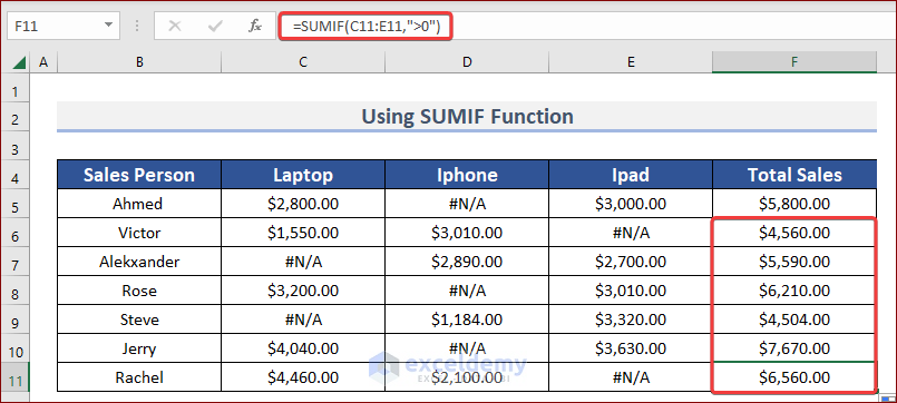
Alternative for Method 1
- You can also use the following formula:
=SUMIF(C5:E5,">0")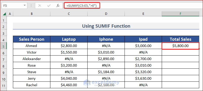
- Use the Fill Handle to AutoFill formula.
Read More: Excel Sum If a Cell Contains Criteria
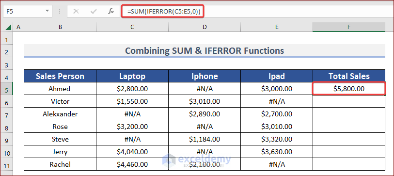
Method 2 – Combine the SUM and IFERROR Function to SUM and Ignore N/A
Steps:
- Apply the following formula in cell F5:
=SUM(IFERROR(C5:E5,0))IFERROR will pass the value of a cell if it’s numeric or return 0 if it encounters a cell with an error, which will be used to sum the cells.
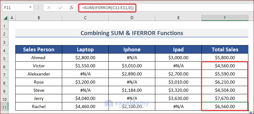
- Use the Fill Handle to AutoFill formula for the rest of the cells in column F.
Alternative for Method 2
- You can also use the following formula:
=SUM(IFERROR(C5:E5,""))
Read More: Sum Formula Shortcuts in Excel
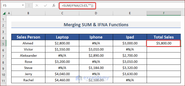
Method 3 – Merge SUM and IFNA Functions to SUM and Ignore N/A
Steps:
- Insert the following formula into F5 and hit Enter.
=SUM(IFNA(C5:E5,""))IFNA specifically checks if the value of the cell is the #N/A error and returns the second argument. Otherwise, it returns the original value.
- Use the Fill Handle to AutoFill formula for the rest of the cells of column F.

Read More: How to Add Specific Cells in Excel
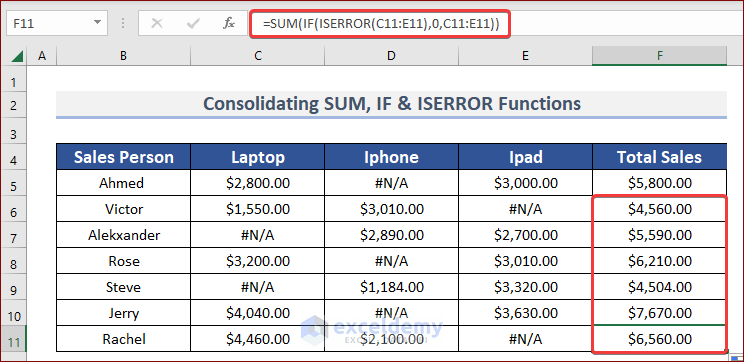
Method 4 – Consolidate SUM, IF, and ISERROR Functions to SUM and Ignore N/A
Steps:
- Insert the following formula into F5.
=SUM(IF(ISERROR(C5:E5),0,C5:E5))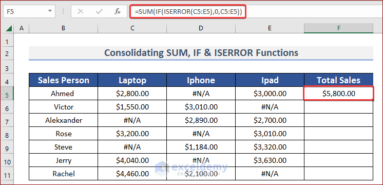
- Hit Enter and use the Fill Handle to AutoFill formula for the rest of the column.
Read More: How to Add Multiple Cells in Excel
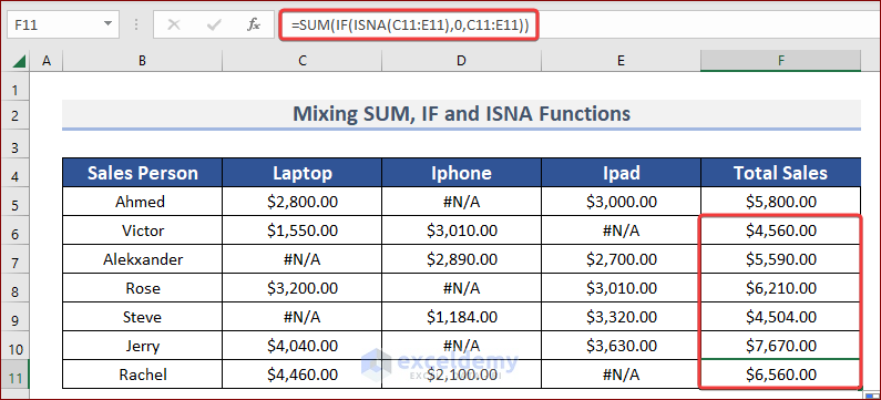
Method 5 – Mix SUM, IF, ISNA Functions to SUM and Ignore N/A
Steps:
- Apply the following formula in F5.
=SUM(IF(ISNA(C5:E5),0,C5:E5))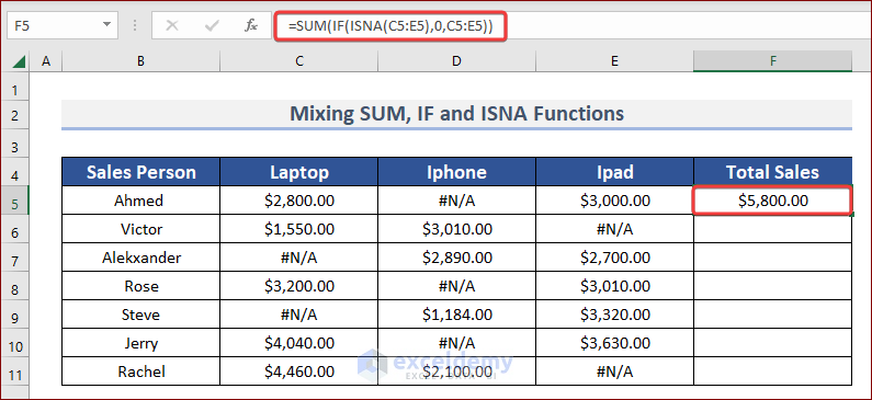
- AutoFill the formula for the rest of the cells of column F.
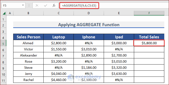
Method 6 – Apply the AGGREGATE Function to SUM and Ignore N/A
Steps:
- Use the following formula in the selected cell (i.e. F5) and hit Enter.
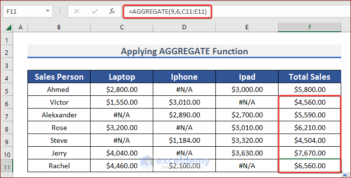
=AGGREGATE(9,6,C5:E5)In the AGGREGATE function, 9 as function_num applies the SUM function, while 6 as option ignores error values.
- AutoFill the rest of the cells in column F.
Read More: How to Sum Range of Cells in Row Using Excel VBA
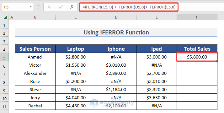
Method 7 – Use the IFERROR Function Multiple Times to SUM and Ignore N/A
Steps:
- Use the following formula in F5 and press Enter.
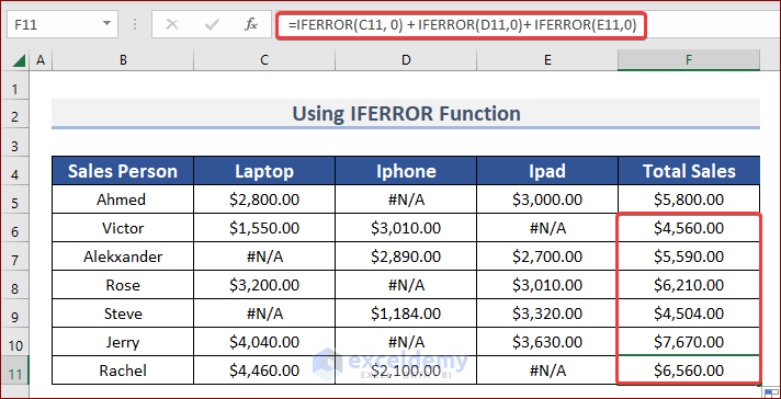
=IFERROR(C5, 0) + IFERROR(D5,0)+ IFERROR(E5,0)This formula manually adds values, so it might be cumbersome to write for larger datasets.
- Use the Fill Handle to AutoFill the formula.
Read More: [Fixed!] Excel SUM Formula Is Not Working and Returns 0
Download the Practice Workbook
Further Readings
- How to Sum Multiple Rows and Columns in Excel
- Sum If a Cell Contains Text in Excel
- How to Sum If Cell Contains Specific Text in Excel
- Sum a Column in Excel
- How to Add Numbers in Excel
- Sum to End of a Column in Excel

