Truncating a number means decreasing the number of digits from the decimal section or from the right side of that number in mathematics. In Excel, sometimes after any calculation, we get a result with large digits in the decimal section. Maybe all the digits are not required. We may require a certain number of digits, or we want the integer part only. Excel has some dedicated functions to perform those tasks. There are also other ways to truncate numbers in Excel. In this article, we will discuss all the methods to truncate numbers in excel with proper illustrations.
How to Truncate Numbers in Excel: 8 Methods
We can truncate numbers from the left or right sides in Excel. There are also options to truncate texts in Excel.

We will truncate numbers using the following dataset. Have a look at the below section for all the methods.
1. Use of TRUNC Function to Truncate Numbers
Here, we will use the TRUNC function. This function can remove all the decimals at a time. Besides, we can also keep a certain number of decimal digits in the numbers. Moreover, there is an option to shorten any number.
📌 Steps:
- Put the following formula based on the TRUNC function on Cell C5.
=TRUNC(B5)
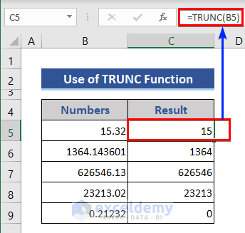
We can see all the decimal digits have been removed from the number.
There is another option in the TRUCN function. We can keep the desired number of decimal digits. Then put that desired number in the formula.
- Look at the formula below used in Cell D5.
=TRUNC(B5,1)

We put 1 in the formula. It means 1 decimal digit will exist in the result.
- We can also shorten the value of a number using this TRUNC function.
- Look at the following formula of Cell E5.
=TRUNC(B5,-1)

We got 10 instead of 15. Because we put -1 in the formula. This reduces the last digit of the integer part of the given number and makes it 0 (“Zero”). If we put -2, that will transform the last two digits of the integer to 0.
Read More: How to Truncate Decimal in Excel
2. Use of INT Function
The INT function just separates the integer part of a number. It is possible to keep any decimal digits when using this INT function.
📌 Steps:
- Look at the following formula used in Cell C5.
=INT(B5)
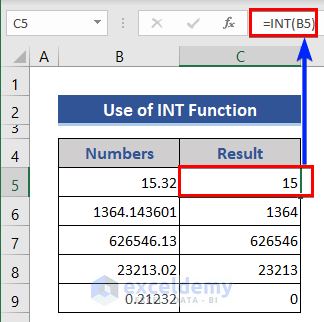
We can see all the numbers truncated by removing the decimal successfully.
3. Use of ROUND Function to Round Off Numbers
The ROUND function rounds off or down a number to a specified number of decimals that mention in the formula. We are not allowed to keep this decimal place argument empty.
📌 Steps:
- Look at the following formula of Cell C5.
=ROUND(B5,1)
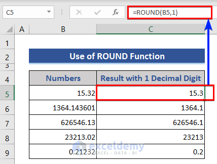
We put 1 in the decimal place. So, we get 1 digit in the decimal section.
If we do not want to remove all the digits from the decimal section, put 0 removing 1.
- Look at the following formula.
=ROUND(B5,0)

All the decimal digits have been removed.
4. Truncate Numbers by Rounding Up
In the previous sections, we truncated the number by the round-down process. But in this section, we will truncate by rounding up the numbers. We will use the ROUNDUP function here.
📌 Steps:
- Look at the formula used on Cell C5.
=ROUNDUP(B5,1)

Here, 15.32 is truncated by rounding up to 15.4. One decimal digit is shown because we put 1 in the second argument.
- If we want to remove all the decimal digits, put 0 on the 2nd Then, the formula becomes:
=ROUNDUP(B5,0)

It rounds up numbers and returns the integer part only.
5. Remove Numbers from the Right and Left Sides
The RIGHT function returns the specified number of characters from the end of a text string.
The LEFT function returns the specified number of characters from the start of a text string.
The FIND function returns starting position of one text string within another text string. This function is case-sensitive.
The LEN function returns the number of characters in a text string.
Previously, we showed how to remove digits from the right side only. Here, we will remove digits from the right and left on both sides.
📌 Steps:
- First, we will use a combination of the LEFT and FIND functions to remove decimal digits from the right side. Look at the formula of Cell C5.
=LEFT(B5,FIND(".",B5)-1)
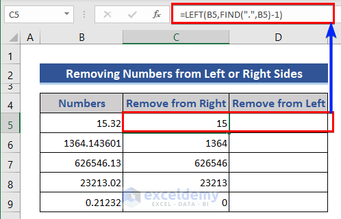
We get the integer numbers only.
- Now, we remove digits from the right side. For that, we will use a combination of RIGHT, LEN, and FIND Put the following formula on Cell D5.
=RIGHT(B5,LEN(B5)-FIND(".",B5))

Here, get the integer numbers only. We separated them from the integer part.
Formula Explanation:
- FIND(“.”,B5)
We want to find the position of the dot (.) in Cell B5.
Result: 3
- LEN(B5)
We want to find out the length of B5.
Result: 32
- LEN(B5)-FIND(“.”,B5)
A subtraction operation is applied here.
Result: 2
- RIGHT(B5,LEN(B5)-FIND(“.”,B5))
This returns the 2 digits from the right side.
Result: 32
Read More: How to Stop Excel from Truncating Text
6. Combination of REPLACE, FIND & LEN Functions
Here, we will use the combination of the REPLACE, FIND & LEN functions to remove numbers from the left side.
📌 Steps:
- Put the following formula on Cell C5.
=REPLACE(B5,FIND(".",B5),LEN(B5)-FIND(".",B5)+1,"")
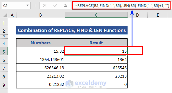
All the decimal digits have been truncated here.
We can also use the SEARCH function despite the FIND function.
REPLACE(B5,SEARCH(".",B5),LEN(B5)-SEARCH(".",B5)+1,"")
Formula Explanation:
- FIND(“.”,B5)
It finds the position of the dot(.) in B5.
Result: 3
- LEN(B5)
Determines the length of B5.
Result: 5
- LEN(B5)-FIND(“.”,B5)+1
Addition and subtraction operations are applied here.
Result: 3
- REPLACE(B5,FIND(“.”,B5),LEN(B5)-FIND(“.”,B5)+1,””)
Replace operation is applied using the values of the previous section.
Result: 15
7. Use of Excel Flash Fill Feature to Truncate Numbers
The Flash Fill is a wonderful feature of Excel. It follows the given sample or sequence and applies that to the rest of the cells.
📌 Steps:
- In the 1st column of the dataset, numbers are given. We want to get only the integers. So, type 15 on Cell C5.
- Then, click on the Flash Fill option of the Data tab.

- Look at the dataset.
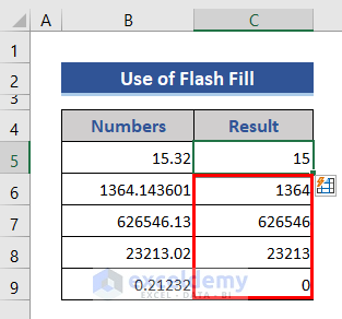
Decimal digits are truncated from the numbers. We can also use a simple Keyboard shortcut Ctrl + E.
8. Use of Text to Columns Wizard
There is another option in Excel to truncate numbers without a formula. This is the Text to Columns feature.
📌 Steps:
- First, select the data range of the Result column.
- Go to the Data tab.
- Choose the Text to Columns feature from the Data Tools group.

- Step 1 of Convert Text to Columns Wizard window.
- Choose Delimited and then click on the Next button.

- In Step 2, mark the Other option and put a dot(.) on the box.
- Again, click the Next button.

- In Step 3, we will skip one column. Then choose the Do not import column (skip).
- Finally, press the Finish button.

- Look at the dataset.

We can see the decimal part has been removed.
How to Truncate Text in Excel
Previously, we showed how to truncate numbers in Excel. Now, we will show how to truncate text in Excel. We will use the combination of LEFT and FIND functions and truncate the 2nd part of the text.
📌 Steps:
- Put the following formula on Cell C5.
=LEFT(B5,FIND(" ",B5)-1)
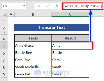
We can see in the Result column only the 1st part is showing.
Read More: How to Truncate Text from Right in Excel
Download Practice Workbook
Download this practice workbook to exercise while you are reading this article.
Conclusion
In this article, we described how to truncate numbers in Excel with and without a formula. We also showed how to truncate texts in Excel. I hope this will satisfy your needs.
Related Articles
- How to Truncate Text in Excel
- How to Truncate Text from Left in Excel
- How to Truncate Date in Excel
- How to Use Truncate in Excel VBA
<< Go Back to Excel TRUNC Function | Excel Functions | Learn Excel
Get FREE Advanced Excel Exercises with Solutions!
