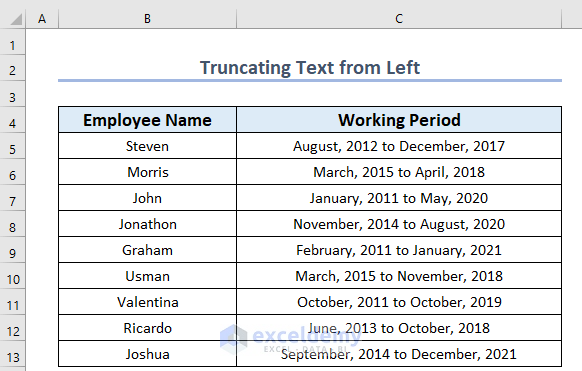
The dataset showcases Employee Name and Working Period.
Method 1 – Using the Excel LEFT Function to Abbreviate Text from the Left
Steps:
- Select a new cell: D5 to keep the truncated text.
- Use the formula below in D5.
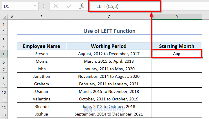
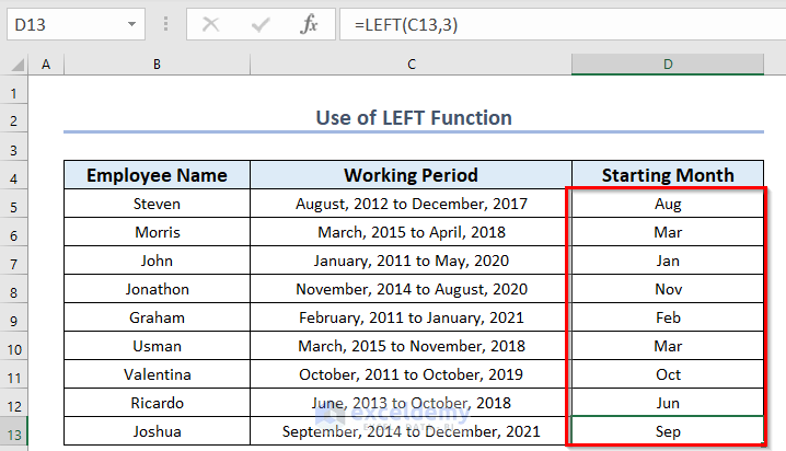
=LEFT(C5,3)The function returns a particular number of characters from the start of the text: 3.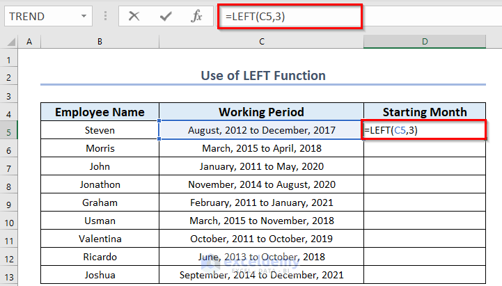
- Press ENTER to see the result.
- Drag down the Fill Handle to see the result in the rest of the cells.
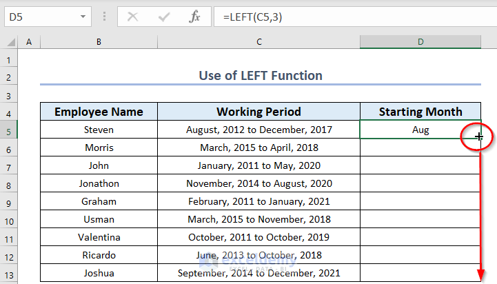
- The joining months of all employees is displayed.
Read More: How to Truncate Text in Excel
Method 2 – Combine the LEFT & LEN Functions to Truncate Text from the Left
Steps:
- Select a new cell: D5 to keep the truncated text.
- Use the formula below:
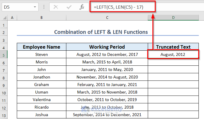
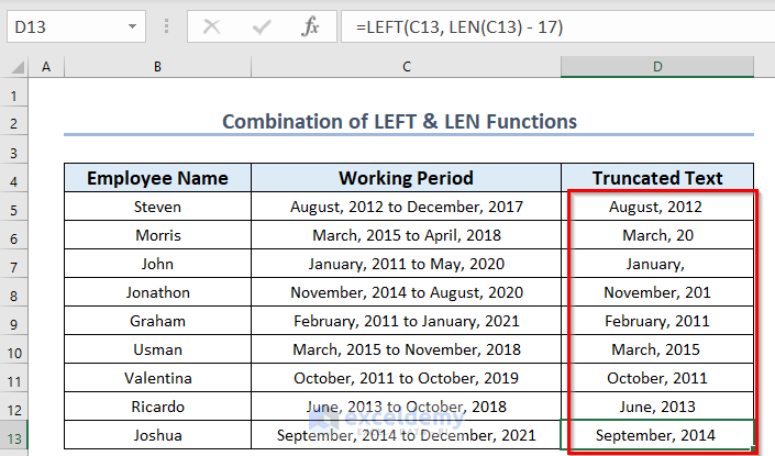
=LEFT(C5, LEN(C5) - 17)- Press ENTER to see the result.
Formula Breakdown
- Here, LEN(C5) returns the total number of characters of the text in C5.
- Output: 30.
- 30-17.
- Output: 13.
- The LEFT(C5,13) function returns a number of characters: 13 characters from the leftmost character of the text in C5.
- Output: August, 2012.
- Drag down the Fill Handle to see the result in the rest of the cells.
- This is the output.
Read More: How to Truncate Text from Right in Excel
Method 3 – Using the MID Function to Truncate Text from the Left in Excel
Steps:
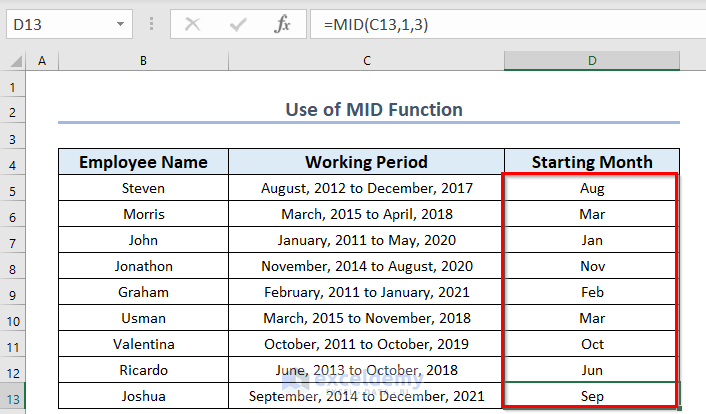
- Select a new cell: D5 to keep the result.
- Use the formula below.
=MID(C5,1,3)The MID function returns a number of characters between the 1st character and the 3rd character in C5.
- Press ENTER to see the result.
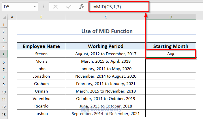
- Drag down the Fill Handle to see the result in the rest of the cells.
- This is the output.
Method 4 – Applying the Excel Flash Fill Feature to Shorten Text from the Left
Steps:
- Enter the target result manually. Here, “Aug”, and “Ma”, and got the suggestion:
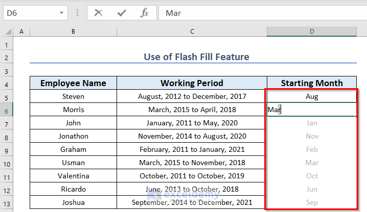
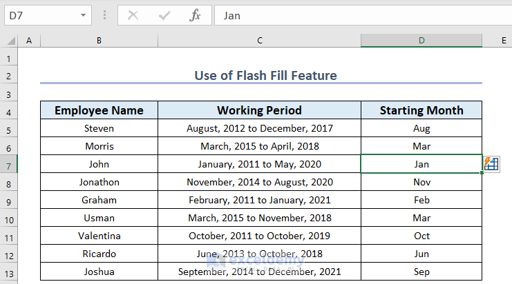
- Press ENTER to see the result.
- This is the output.
Read More: How to Stop Excel from Truncating Text
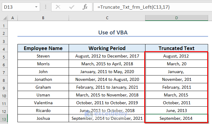
Method 5 – Truncate Text from the Left applying a User-Defined Function in Excel
Steps:
- Go to the Developer tab >> select Visual Basic.
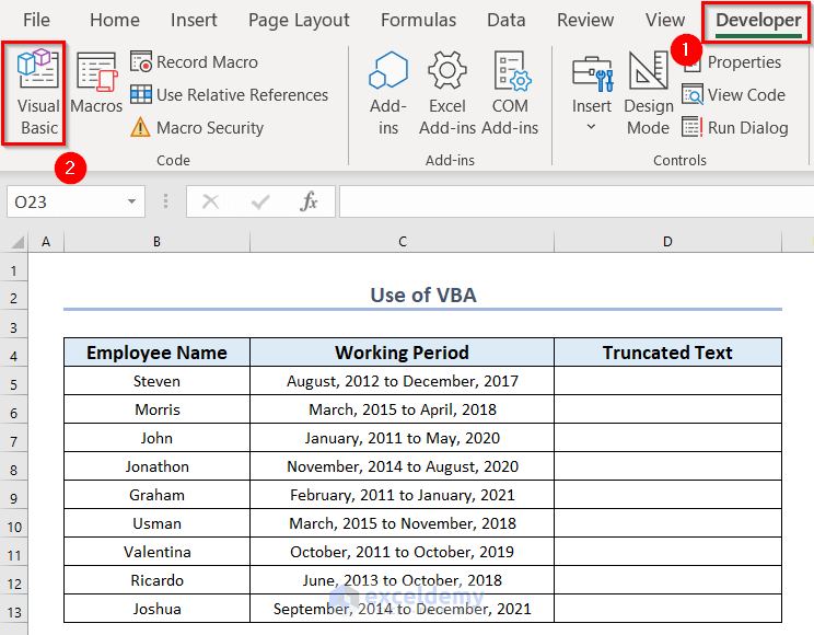
- In Insert >> select Module.
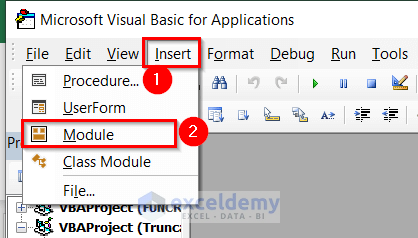
- Enter the following Code in the Module.
Function Truncate_Txt_frm_Left(my_Text As String, removed_num_of_string As Long)
  Truncate_Txt_frm_Left = Left(my_Text, Len(my_Text) - removed_num_of_string)
End Function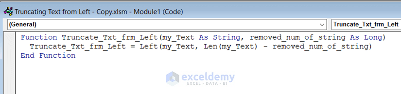
Code Breakdown
- creates a Function: Truncate_Txt_frm_Left.
- declares the variable my_Text as a String to call the text, and another variable removed_num_of_string as Long to insert a number.
- With the Left and Len functions, a function was created: Truncate_Txt_frm_Left.
- Save the code by pressing CTRL+S ( .xlsm).
- Go to the Excel worksheet.
Steps:
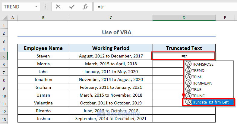
- Select a cell to keep the result. Here, D5.
- Enter “=tr” to find your defined function.
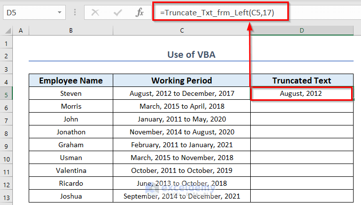
- Use the formula in D5.
=Truncate_Txt_frm_Left(C5,17)The function returns a number of characters from the start of the text: 17 characters from the leftmost character in C5.
- Press ENTER to see the result.
- Drag down the Fill Handle to see the result in the rest of the cells.
- This is the output.
Read More: How to Use Truncate in Excel VBA
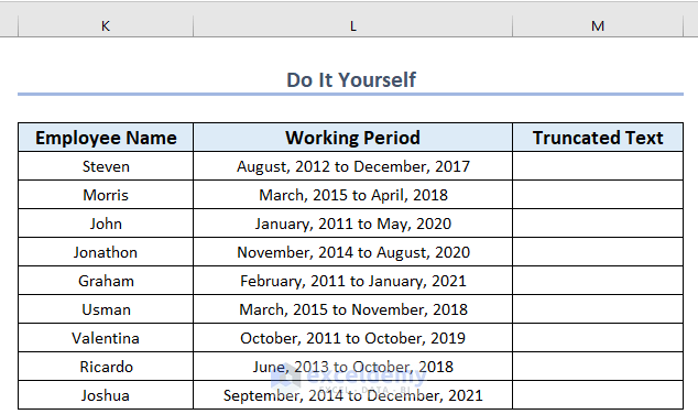
Practice Section
Practice here.
Download Practice Workbook
Download the practice workbook.
Related Articles
<< Go Back to Excel TRUNC Function | Excel Functions | Learn Excel
Get FREE Advanced Excel Exercises with Solutions!
