How to Truncate Text in Excel (6 Suitable Methods)

When you have a big dataset with text as a cell value, then you may need to truncate text in Excel. So, if you are looking for how to truncate text in Excel, then you have come to the right place. Today, in this article, I’m going to explain how to truncate text in Excel.

Furthermore, for conducting the session, I will use Microsoft 365 version.

How to Truncate Text in Excel: 6 Methods

Here, I will demonstrate 6 suitable methods with detailed steps on how to truncate text in Excel. For your better understanding, I am going to use the following dataset. Which contains two columns. Those are Employee Name and Working Period. The dataset is given below.

1. Applying LEFT Function to Truncate Text in Excel

You can apply the LEFT function to truncate text in Excel. In my dataset, the working period of every employee is given. At this time, suppose, I want to find out only the joining month of every employee. So, I need to truncate the whole working period into the starting month. Now, follow the steps given below.

Steps:

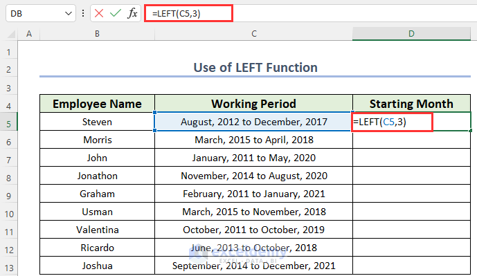
• Firstly, you must select a new cell D5 where you want to keep the result.
• Secondly, you should use the formula given below in the D5 cell.

Here, in this formula, I have used only the LEFT function. This function will return a particular number of characters from the start of the text. Where C5 is that text and it will return the first 3 characters.

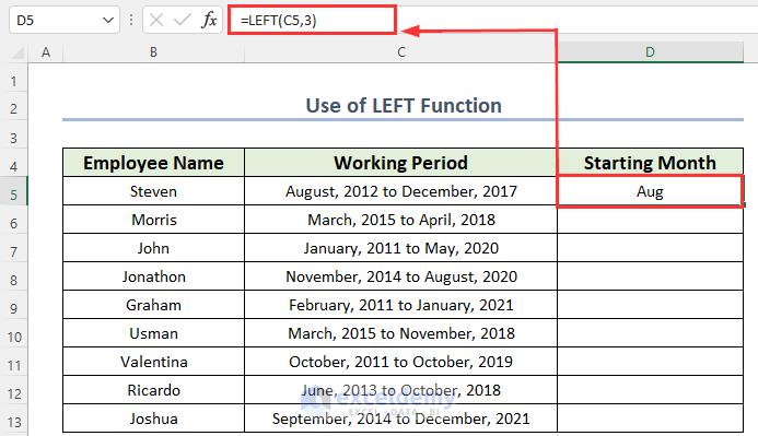
• After that, you must press ENTER to get the result.

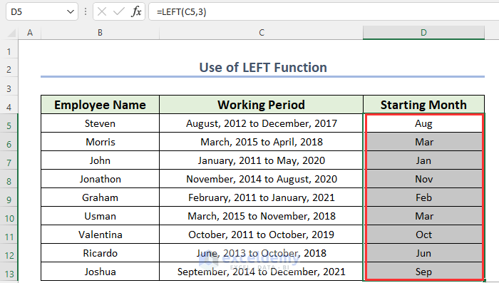
• Now, you can drag the Fill Handle icon to autofill the corresponding data in the rest of the cells D6:D13.

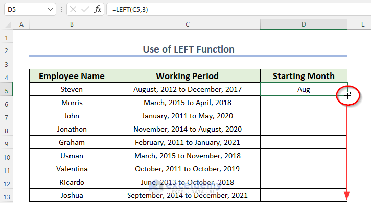
Lastly, you will get all the joining months of employees.

Read More: How to Truncate Text from Left in Excel

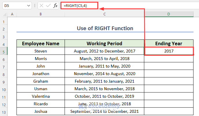
2. Employing RIGHT Function for Truncating Text

You can apply the RIGHT function to truncate text in Excel. Through my dataset, you can see the working period of every employee. At this time, suppose, you want to find out only the ending year of every employee. So, you need to truncate the whole working period into the ending year. Now, follow the steps given below.

Steps:

• Firstly, you must select a new cell D5 where you want to keep the result.
• Secondly, you should use the formula given below in the D5 cell.

Here, in this formula, I have used only the RIGHT function. This function will return a particular number of characters from the end of the text. Where C5 is that text and it will return the last 4 characters.

• Thirdly, press ENTER to get the result.

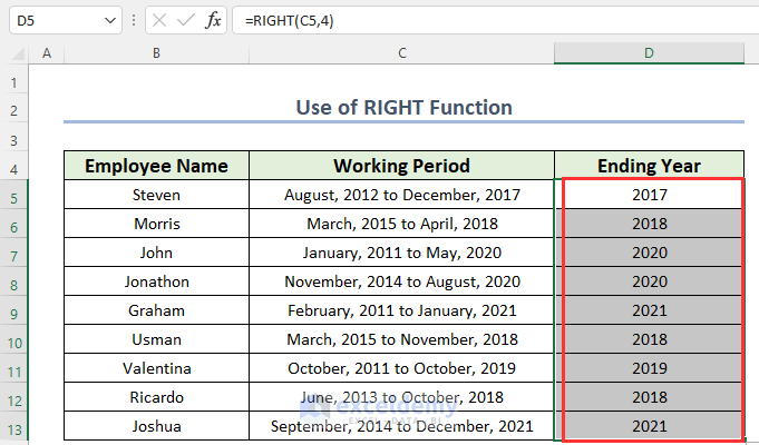
• Now, you can drag the Fill Handle icon to autofill the corresponding data in the rest of the cells D6:D13.

Finally, you will get all the ending years of employees.

Read More: How to Truncate Text from Right in Excel

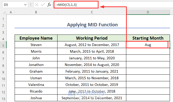
3. Using MID Function to Truncate Text in Excel

Here, you can apply the MID function to truncate text in Excel. Through my dataset, you can see the working period of every employee. At this time, suppose, you want to find out only the joining month of every employee. So, you need to truncate the whole working period into the starting month. Now, follow the steps given below.

Steps:

• Firstly, you must select a new cell D5 where you want to keep the result.
• Secondly, you should use the formula given below in the D5 cell.

Here, in this formula, I have used only the MID function. This function will return a particular number of characters from a defined character place in the text. Where C5 is that text and it will return from the 1st character to the 3rd character.

• Thirdly, press ENTER to get the result.

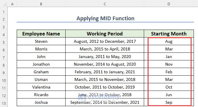
• Then, you can drag the Fill Handle icon to autofill the corresponding data in the rest of the cells D6:D13.

Finally, you will get all the starting months of employees.

Read More: How to Truncate Date in Excel

4. Applying Text to Columns Feature in Excel

At this time, suppose, you want to find out all the details about the employee’s working period like when an employee joined when he left the job, etc. Basically, you want to keep these details in particular columns. So, it would be best if you truncated the text in Excel. Furthermore, to do so, I will use the Text to Columns feature.

• Here, you have to define the column header. Below, I have attached an image.

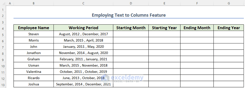
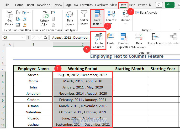
• Firstly, select cell C4:C13.
• Secondly, from the Data tab >> go to the Data Tools option.
• Finally, choose the Text to Columns feature.

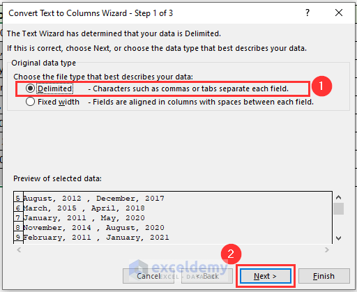
At this time, you will see a new dialog box named Convert Text to Columns Wizard – Step 1 of 3.

• Then, you have to mark Delimited – Characters such as commas or tabs separate each field.
• After that, press Next.

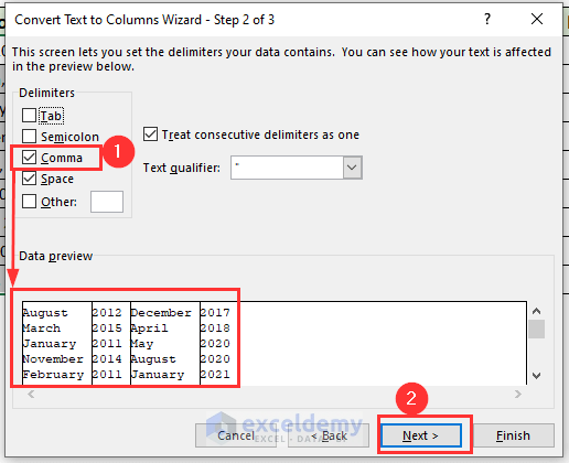
Subsequently, you will see another dialog box named Convert Text to Columns Wizard – Step 2 of 3.

• Now, you have to mark Comma, Space which is under the Delimiters. Here, you can immediately see the modified data in the Data preview box.
• Then, press Next.

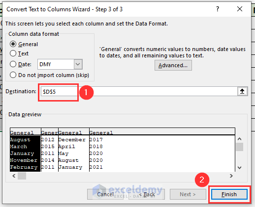
Again, you will see a dialog box named Convert Text to Columns Wizard – Step 3 of 3.

• Firstly, you may keep General which is under the Column data format. Here, you should mark the Column data format based on your data type.
• Then, choose the Destination.
• Finally, press Finish.

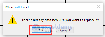
At this time, you will see the warning from Microsoft Excel.

• Then, press OK on it.

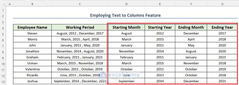
Lastly, you will see the truncated text in separate columns.

5. Use TEXTSPLIT Function to Split Text in Excel

Like the previous one, suppose, you want to find out all the details about the employee’s working period like when an employee joined when he left the job, etc. Basically, you want to keep these details in particular columns. So, it would help if you truncated the text in Excel. Furthermore, to do so, I will show you another way here. Actually, you can do this by using the TEXTSPLIT function.

• Firstly, you have to define the column header. Below, I have attached an image.
• Secondly, you must select a new cell D5 where you want to keep the result.
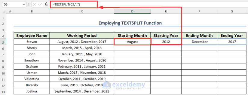
• Thirdly, you should use the formula given below in the D5 cell.

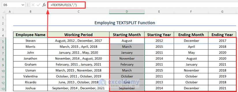
Here, in this formula, I have used only the TEXTSPLIT function. Actually, this function will separate a text based on a defined delimiter. Where C5 is that text and it will separate the text depending on comma (,). Furthermore, you must use an inverted comma to specify the delimiter.

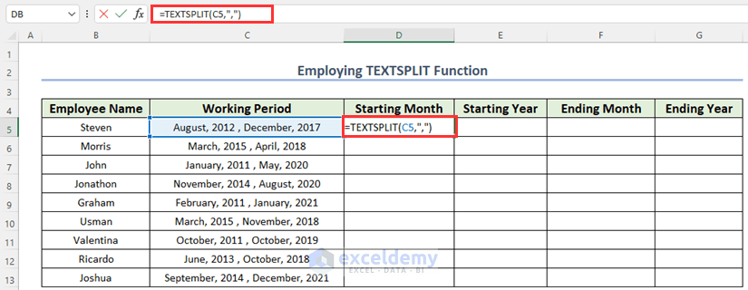
• Then, press ENTER to get the result.

As a result, you will see all the information about Steven in separate columns.

• Now, you can drag the Fill Handle icon to autofill the corresponding data in the rest of the cells D6:D13.

Finally, you will get all the truncated text in separate columns.

Read More: How to Stop Excel from Truncating Text

6. Employing Excel Flash Fill Feature to Truncate Text

In this method, I’m going to use the Flash Fill feature to truncate text in Excel. Actually, this is an interesting and simple way. Basically, you will truncate the text into separate columns by following a pattern. Now, let’s see the steps given below.

Steps:

• Firstly, you have to write the target result manually up to which you can see Excel’s suggestion. For example, I have written “Aug”, and “Ma”, and then I got the suggestion.

Actually, you have to do this to show Excel a pattern. So, when Excel understands your pattern then Excel will suggest you the output. Below, I have attached the image.

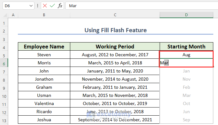
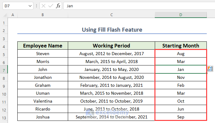
• Subsequently, press ENTER to get the result.

Finally, you will get all the starting months of employees.

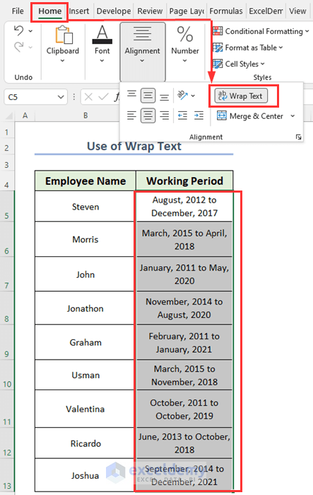
How to Wrap Text in Excel Using Shortcuts

Here, in this section, I will show you how to wrap text in Excel using the Keyboard shortcuts. Suppose you have the following dataset. In the column named working period, the text strings are large and so you want to wrap text to understand the dataset. Actually, in this case, you may expand the column and easily see the whole text. But whenever you have long enough text then you may need to wrap the text.

The steps are given below.

Steps:

• Firstly, select the dataset.
• Secondly, press AIT+H+W.

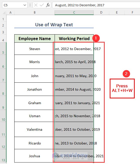
Lastly, you will see that all the texts are wrapped. Furthermore, from the Home tab >> you can check whether the texts are wrapped or not.

Practice Section

Now, you can practice the explained method by yourself.

Download Practice Workbook

You can download the practice workbook from here:

Conclusion

I hope you found this article helpful. Here, I have explained 6 suitable methods to truncate text in Excel. Hope you can solve all the problems regarding the truncating text. Please, drop comments, suggestions, or queries if you have any in the comment section below.

Related Articles

• How to Truncate Decimal in Excel
• Truncate Numbers in Excel
  
• How to Use Truncate in Excel VBA

<< Go Back to Excel TRUNC Function | Excel Functions | Learn Excel