We often use decimal values in Excel. For practical purposes, we need to modify these decimal values. And Excel can do this modification very efficiently. This article will show you how you can truncate decimal values in Excel. There are many ways to change decimal numbers. This article especially deals with how to reduce decimal values in Excel. For that, we will use several functions such as INT, TRUNC, ROUND, ROUNDUP, ROUNDDOWN, and the in-built Number Format.
1. Using In-Built Number Format to Truncate Decimal
You can easily truncate decimal values in Excel using the in-built Number Format feature. Let’s see the method.
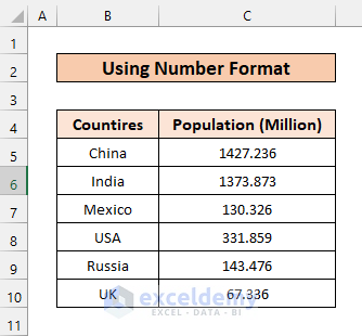
We have taken a dataset of countries and their total population. The population is in the form of 3-point decimals. Now we will truncate this data using this feature.
Steps:
➤ First, select the data range C5:C10 that you want to truncate.
➤ Then, go to Home > Number and click on the Decrease Decimal icon.

So, all the numbers are reduced to 2-point decimal.

Read More: How to Truncate Numbers in Excel
2. Applying INT Function to Truncate Decimals
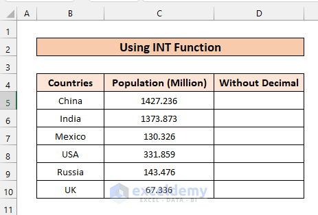
Now we will truncate decimals using the INT function. This function will only give us an integer value and the decimal portion will be dissolved.
We added a new column on the right side of the Population column. In this new column, we will use the function.
Steps:
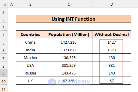
➤ Write the following formula in D5 and press ENTER.
=INT(C5)This equation takes a number and gives an integer output.

So, we get our first truncated number which is 1427.
➤ Now, hold and drag the D5 cell downward.

Thus, we get all the truncated numbers.
3. Utilizing the TRUNC Function to Truncate Decimal
As the name suggests, the TRUNC function is especially used to truncate decimal numbers. In this method, we will find out 1st and 2nd decimal values using this function.
For that, we have added two columns; 1st Decimal and 2nd Decimal.

Steps:
➤ Write the following formula in D5 and press ENTER.
=TRUNC(C5,1)In this formula,
C5:- the cell we want to truncate
1:- number of digits after decimal

So the decimal value is reduced to the 1st decimal.
➤ Now, hold and drag the D5 cell downward.

And, we have all the decimal values reduced to 1st decimal.

Again, we are going to find out the 2nd decimal of these data.
➤ Write the following formula in E5 and press ENTER.
=TRUNC(C5,2)C5:- the cell we want to truncate
2:- number of digits after the decimal

So, we have got a second decimal for the first number.
➤ Now, hold and drag the E5 cell downward.

Thus, all the decimal values are reduced to 2nd decimal.

Read More: How to Truncate Date in Excel
4. Using ROUND Function
The ROUND function gives the nearest higher integer value. Its output is somewhat different from the previously shown methods. Let’s see how this is done.
Steps:
➤ Write the following formula in D5 and press ENTER.
=ROUND(C5,1)In this equation,
C5 is the cell we want to truncate.
1 is the number of digits we want after the decimal.

So we have our first truncated decimal.
➤ Now, hold and drag the D5 cell downward.

Thereby, all the decimal values are reduced to 1st decimal.

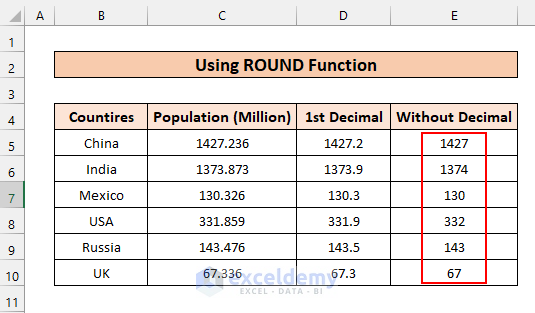
Now, let’s say we don’t want any digit after the decimal.
➤ So write the following formula in E5 and press ENTER.
=ROUND(C5,0)C5 is the cell we want to truncate.
0 is the number of digits we want after the decimal.
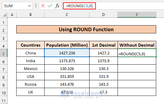
So we get our first integer value.
➤ Now, hold and drag the E5 cell downward.

Thereby we have all the decimal values reduced as integers.
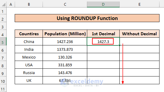
5. Using the ROUNDUP Function to Truncate Decimal
The ROUNDUP function rounds the numbers to the next higher possible value. This method will take the value from column C and round them in two different criteria. Let’s see how it can be done.
Steps:
➤ First, write the following formula in D5 and press ENTER.
=ROUNDUP(C5,1)C5 is the cell we want to truncate.
1 is the number of digits we want after the decimal.

So, we get our first modified value. You can see that the outcome value is higher than the original one.
➤ Now, hold and drag the D5 cell downward.
Thus, we have all the decimals modified using the function.

Now, we will reduce these decimals into integers.
➤ Write the following equation in E5 and press ENTER.
=ROUNDUP(C5,0)C5 is the cell we want to truncate
0 is the number of digits we want after the decimal.
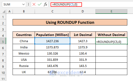
So, we have our first value rounded up.
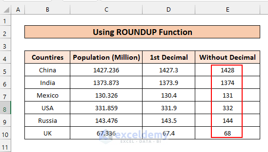
➤ Now, hold and drag the E5 downwards.

Thereby we get all the rounded-up values.
Read More: How to Truncate Text from Right in Excel
6. Using ROUNDDOWN Function
The ROUNDDOWN function is just the opposite of the previous method. This function gives us the nearest lower value for a given number.
Steps:
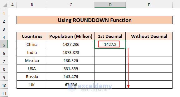
➤ Write the following equation in D5 and press ENTER.
=ROUNDDOWN(C5,1)C5 is the cell we want to truncate
1 is the number of digits we want after the decimal.

Thus, we have got our first rounded-down number.
➤ Now, hold and drag the D5 cell downward.
Thereby, we have all the decimal values rounded down to 1st decimal.

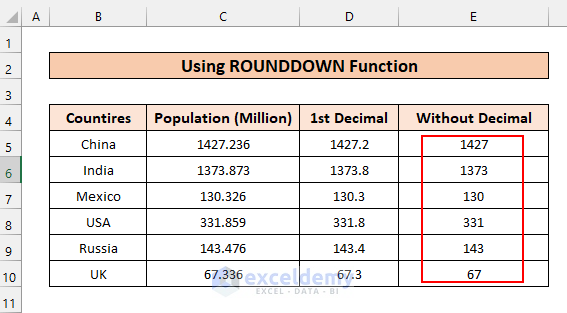
Again, we want to get integer values using this very function.
➤ Write the following equation in E5 and press ENTER.
=ROUNDDOWN(C5,0)C5 is the cell we want to truncate
0 is the number of digits we want after the decimal.

So, we get our first rounded-down value.
➤ Now, hold and drag the E5 cell downward.

Thus, all the decimal values are rounded down as integers.
Practice Section
You can download the practice workbook from the download section and practice yourself.

Download Practice Workbook
You can download and practice this workbook.
Conclusion
So, we have learned 6 easy methods of truncating decimals in Excel. We hope the content of this article has been helpful to you and you will be able to truncate decimals in Excel without any problem. If you have any queries or suggestions, feel free to mention them in the comment section.
Related Articles
- How to Truncate Text in Excel
- Stop Excel from Truncating Text
- How to Truncate Text from Left in Excel
- How to Use Truncate in Excel VBA
<< Go Back to Excel TRUNC Function | Excel Functions | Learn Excel
Get FREE Advanced Excel Exercises with Solutions!
