While working with numbers that have decimal parts in Excel we need to round down those numbers for ease of calculation or decimal parts of the numbers are not required. We can easily round down the number with decimal parts or even the integers to the nearest 10th, 100th, or 1000th places if we know how to use Excel ROUNDDOWN function. In this article, I will explain 5 simple ways how to use Excel ROUNDDOWN function so you can easily round down numbers according to your convenience
Introduction to the ROUNDDOWN Function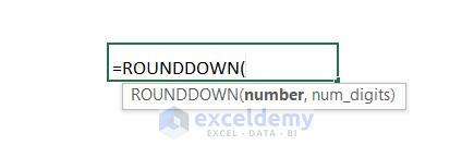 Function Objective:
Rounds a number down, toward zero.
Syntax:
=ROUNDDOWN(number, num_digits)Argument Explanation:
| Argument | Required/Optional | Explanation |
|---|---|---|
| number | Required | Any real number that you want to be rounded down. |
| num_digits | Required | The number of digits to which you want to round number. |
Return Parameter:
The rounded down value of the first argument(number) towards zero.
How to Use ROUNDDOWN Function in Excel: 5 Suitable Methods
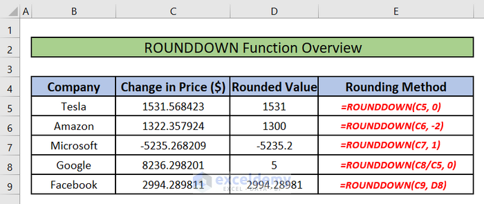
Let’s assume a scenario where we are working with the prices of shares of various companies enlisted in NASDAQ. The share prices of these companies have large decimal values and, in some cases, numbers themselves are too large to work with. We will learn 5 easy methods using Excel ROUNDDOWN function to round down these numbers. By the end of this article, we will be able to round down numbers to a specific decimal point, to the left of the decimal point, negative numbers, nesting inside the ROUNDDOWN function, and round down using variable digits to round the number to that digit.
1. Rounded Down to the Right of the Decimal Point
You might want to round down the numbers to a specific number of digits right to the decimal point. You can do that easily by following these steps:
Step 1:
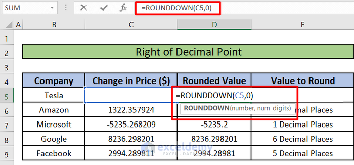
- First, select the cell where you want the rounded value. It can be the cell whose value you want to be rounded down. In that case, the value of that cell will be updated after you have applied the ROUNDDOWN. You can also use another cell to store the Rounded Down value so the actual will be preserved. In our Excel worksheet, we have selected cell D5 to store our Rounded Down value.
Step 2:
- We want to round down the Changes in the Price of shares for Tesla. That is cell C5. So, in selected cell D5 or the Insert Function bar, we will write down the following formula.
=ROUNDDOWN(C5,0)Here,
C5 = Number = The number we want to round down
0 = num_digits = The number of digits to which we want to round number. We want to round our number to zero decimal places.
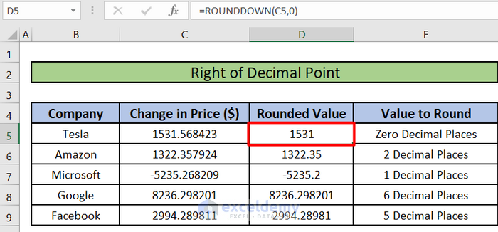
- After entering the above formula, if we press enter we will see that the rounded down value of C5 is showing in cell D5 under the column named Rounded Value.
2. Round Down to Left of the Decimal Point
You might want to round down the numbers left of the decimal points. This can be done following the same methods. But to round down the number left of the decimal point you have to put an extra negative sign (–) in from of the second argument Num_digits. You can round down to the nearest 10, 100, 1000, etc.
Step 1:
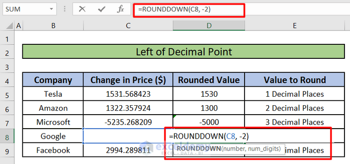
- We want to round down the value of cell C8 (Change in Price of shares for Google) to the nearest 100. That means we want to round down the value 2 decimal places to the left of the decimal points. We will select cell D8 to show our rounded-down value of cell C8.
Step 2:
- After selecting D8, we will write down the following formula in that cell or the Insert Function
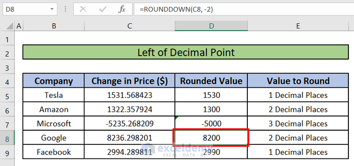
=ROUNDDOWN(C8,-2)We have put -2 as the second argument (num_digits) in the function ROUNDDOWN. We want to round down the value left of the decimal point. So we have added an extra negative sign in front of the 2.
- After entering the above formula, if we press enter we will see that the rounded down value of C8 is showing in cell D8 under the column named Rounded Value.
3. ROUNDDOWN Negative Numbers in Excel
If we need to round down any negative numbers, that can also be done using the same formula.
Step 1:
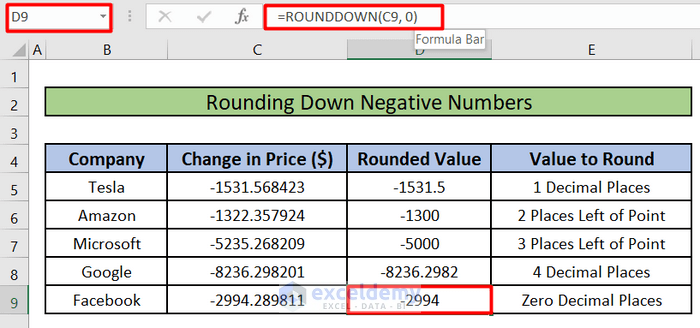
- Let’s say, we want to round down the value of cell C9 (Change in Price of shares for Facebook). It is a negative value that means the price of the share fell. We want to round down the value to 0 decimal places. We will select cell D9 to show our rounded-down value of cell C9.
Step 2:
- After selecting D9, we will write down the following formula in that cell or the Insert Function formula bar:
=ROUNDDOWN(C9,0)- Upon pressing ENTER, We will find out that the rounded-down negative value of cell C9 is shown in cell D9.
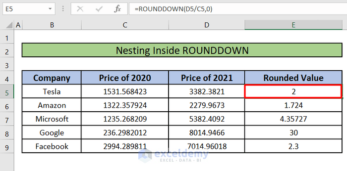
4. Nesting inside the ROUNDDOWN Function
Other operations and functions can be nested inside the ROUNDDOWN function. For example, we might want to divide the share price of Tesla in 2021 (cell D5) by the price in 2020 (cell C5) to find out how much the price has changed over the year. We might need to round the value to zero decimal places to clearly understand the change.
Steps:
- First, we will select cell E5 to show the rounded value in that cell. In that cell or the Formula Bar, we will write the following formula:
=ROUNDDOWN(D5/C5,0)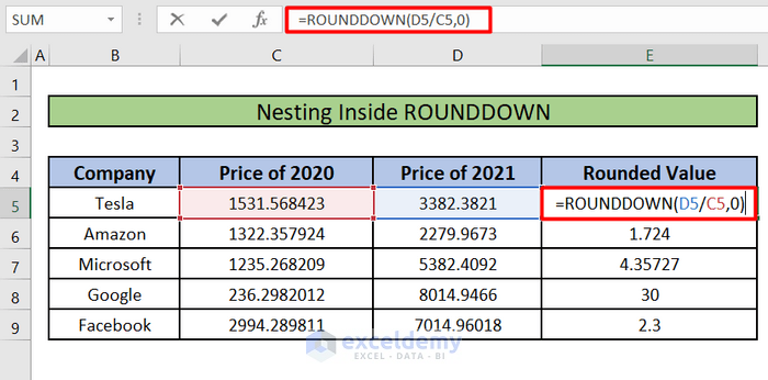
- Upon pressing ENTER, we will find out that the rounded-down value is shown in cell E5.
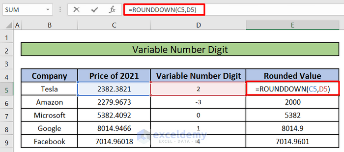
5. ROUNDDOWN with Variable Number Digits in Excel
We might want to round down different values to a different number of digits. To do that, we can store the Numbers to be rounded down in one column and the Num_digits in another column.
Steps:
- In the worksheet below, we have created a column titled Variable Number Digit. This column will store the different num_digits (Second Argument of the Function).
- In the Rounded Value column, we will select cell E5 and write the following formula:
=ROUNDDOWN(C5,D5)C5 = Number = Number we want to round down
D5 = num_digits = The number of digits to which we want to round number
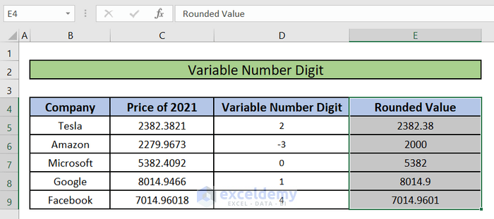
- After pressing ENTER, the rounded-down value will be shown in cell E5.
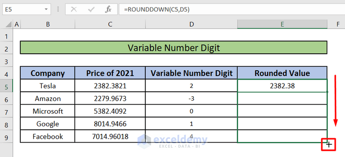
- ROUNDDOWN function will round every cell below E5 in the Rounded Value column according to the respective number in the same row under the Variable Number Digit
Things to Remember
- ROUNDDOWN behaves like the ROUND function, except that it always rounds a number down.
- If num_digits is greater than 0 (zero), then the function will round the number down to the specified number of decimal places.
- It will round down the number to the nearest integer if num_digits equals to 0
- If num_digits is less than 0, then the function will round the number down to the left of the decimal point
Download Practice Workbook
Download this practice book to exercise the task while you are reading this article.
Conclusion
In this article, we have learned 5 easy ways to round down the number in Excel. I hope now you have a clear idea of how to use the Excel ROUNDDOWN function to round the number right and left of the decimal point, round negative numbers, how to nest other operations and functions inside the will round down ROUNDDOWN function, and how to use variable num_digits to round down different numbers to different values. If you have any queries or recommendations about this article, please do leave a comment below. Have a great day!!!
<< Go Back to Excel Functions | Learn Excel
Get FREE Advanced Excel Exercises with Solutions!
