Correlation is a type of measure, which mainly uses to show the variation between two data. It also describes the strength and direction of two variables. People mainly use these correlation features in statistics, economics, and social sciences for getting relations in business plans, budgets, and so on. If you are facing any difficulties to do and are interested to know how to do correlation in Excel, then follow us.
What Is Correlation?
Correlation is a non-dimensional value. It shows us the relationship between two variables. In addition, it provides us with an indication of the relationship among those variables by evaluating and relating the variance of each variable. Correlation contains two major functions of statistical calculation. They are Covariance and Standard Deviation. The range of the correlation’s value moves between -1 to +1. The formula of correlation is:
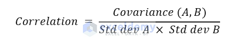
Here, A and B are two different variables.
Let’s explain the whole idea with a simple mathematical example.
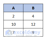
We have 3 values of variables A and B. The values are shown below:
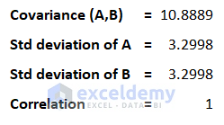
Now, according to the formula calculate the value of Covariance(A, B), Std deviation of A, and Std deviation of B. Put those values in the equation shown above. You will get the value of Correlation.
How to Do Correlation in Excel: 3 Easy Methods
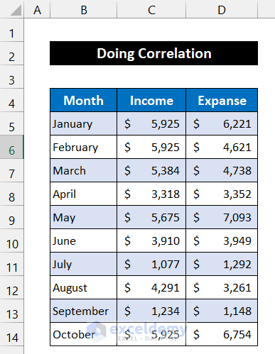
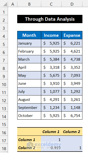
For determining the value of the correlation of two variables, we are considering a dataset where the income and expense of a person for the first 10 months are shown. The name of the months is in column B, and the income and the expanse are in columns C and D respectively. So, we can say that our dataset is in the range of cells B4:D14.
1. Using CORREL Function
In this method, we are going to use the CORREL function to calculate the value of the correlation of our dataset. Our dataset is in the range of cells B4:D14 and the value of the correlation will be in cell C16. The steps of this method are given below:
📌 Steps:
- At first, select cell C16.
- Now, write down the following formula in the cell.
=CORREL(C5:C14,D5:D14)
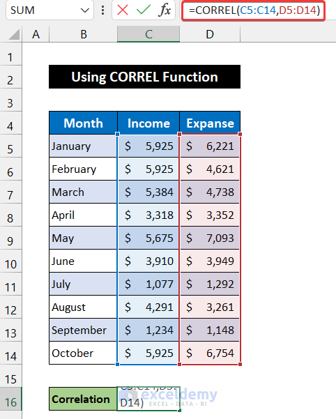
- Press the Enter key on your keyboard to get the result.
- You will see the value correlation of our dataset is shown in cell C16.
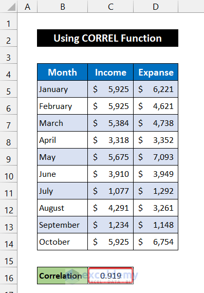
💬 Explanation of the Value for Correlation Used in the Dataset
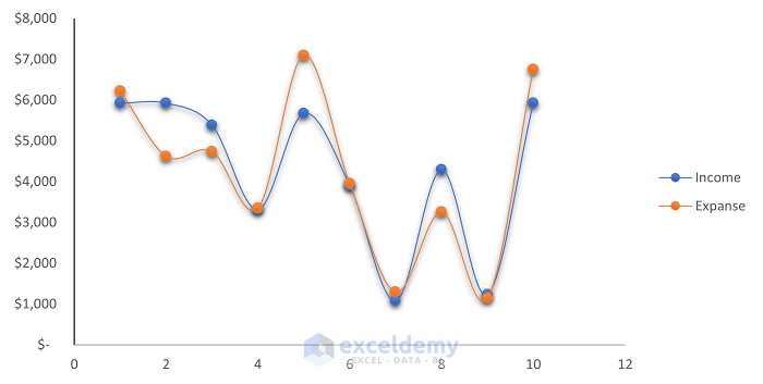
The value of correlation shows us the strength of the relationship between the values of two variables. So, the value of 0.919 indicates that for every row the values are 0.919 times each other. Moreover, this value is the ratio of the covariance of both variables and the multiplication of the standard deviation of Income and the standard deviation of Expanse. A graph is displayed below for a better understanding of this feature.
Finally, we can say that our formula worked successfully and we can estimate the value of the correlation.
2. Applying PEARSON Function
In the following approach, we will use the PEARSON function to calculate the value of the correlation. Our dataset is in the range of cells B4:D14 and the value of the correlation will be in cell C16. The procedure of this method is given as follows:
📌Steps:
- First of all, select cell C16.
- Then, write down the following formula into the cell.
=PEARSON(C5:C14,D5:D14)
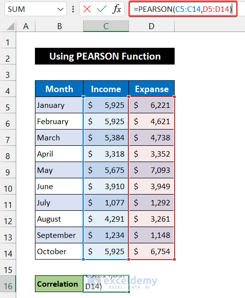
- After that, press the Enter key.
- You will get the value correlation of our dataset is showing in cell C16.
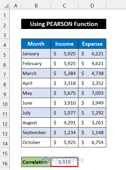
💬 Explanation of the Value for Correlation Used in the Dataset
We know that the value of correlation helps us to understand the strength of the relationship between the values of two variables. For our dataset, the value of 0.919 indicates that for every row the values are 0.919 times each other. Besides it, this value is the ratio of the covariance of both variables and the multiplication of the standard deviation of Income and the standard deviation of expense. A graph is displayed below for a better understanding of this feature.
Thus, we can say that our formula worked perfectly and we are able to do correlation in Excel.
Read More:
3. Use of Excel’s Built-in Data Analysis Feature
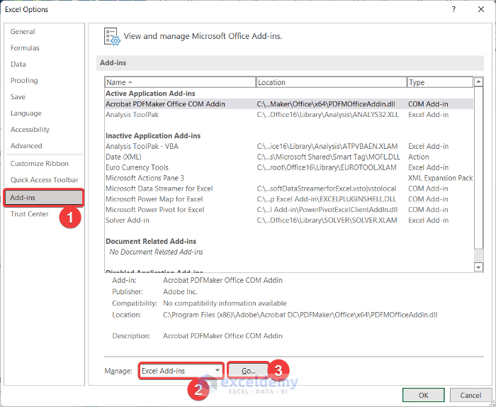
In this process, we will use Excel’s built-in Data Analysis features to do correlation in the Excel dataset. To use this feature, we have to enable the Data Analysis option from Excel’s built-in Add-ins. Our dataset is in the range of cells B4:D14 and the result will be in the range of cells B16:D18. The process is explained below step by step:
📌 Steps:
- To enable the Data Analysis option, first select File > Options.

- A dialog box called Excel Options will appear.
- In this box, select the Add-ins option.
- After that, choose the Manage option as Excel Add-ins and click Go.
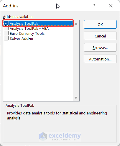
- Another dialog box entitled Add-ins will appear.
- Check the Analysis ToolPak option.
- Finally, click OK.
- You will see a new group called Analysis added in the Data tab.
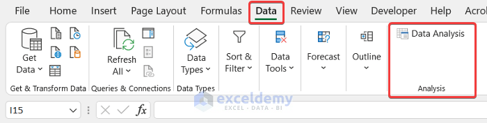
- Now, select the Data Analysis option from the Analysis group.
- A dialog box titled Data Analysis will appear.
- Then, choose the Correlation option and click OK.
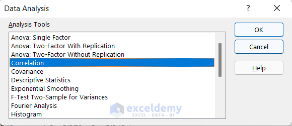
- Another dialog box called Correlation will come.
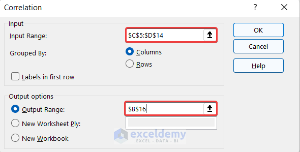
- After that, set the Input Range as $C$5:$D$14, selecting through your mouse.
- Choose the Output options as Output Range and write your desired cell. In our case, we choose cell $B$16.
- Al last clicks the OK option.
- Finally, you will see the value of correlation is showing in the range of cells B16:D18.
💬 Explanation of the Value for Correlation Used in the Dataset
The value of correlation indicates the strength of the relationship between the values of two variables. Thus, the value of 0.919 in cell B18 indicates that for every row the values are 0.919 times each other. Besides it, the value of B17 and C18 shows the correlation value against their own columns, thus those value returns 1. This value is the ratio of the covariance of both variables and the multiplication of the standard deviation of Income and the standard deviation of Expanse.
So, we can say that our approach worked successfully and we are able to do correlation in Excel.
Read More:
Download Practice Workbook
Download this practice workbook for practice while you are reading this article.
Conclusion
That’s the end of this article. I hope that this content will be helpful for you and you will be able to do correlation in your Excel workbook. If you have any further queries or recommendations, please share them with us in the comments section below.
Excel Correlation: Knowledge Hub
- How to Calculate Partial Correlation in Excel
- How to Calculate Cross-Correlation in Excel
- How to Calculate Correlation between Two Stocks in Excel
- How to Do Correlation and Regression Analysis in Excel
- How to Interpret Correlation Table in Excel
- How to Make a Correlation Matrix in Excel
- How to Make Correlation Graph in Excel
- How to Make a Correlation Scatter Plot in Excel
- How to Calculate Spearman Correlation in Excel
- How to Calculate P Value for Spearman Correlation in Excel
- How to Show Relationship Between Two Variables in an Excel Graph
- How to Calculate Correlation Coefficient in Excel

