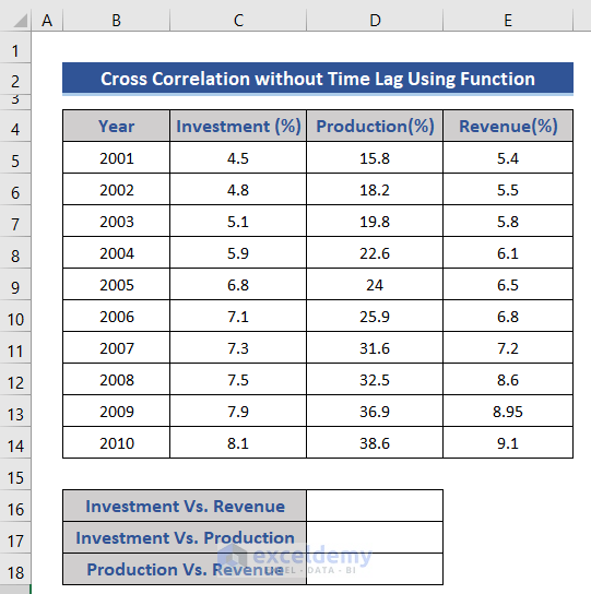
Method 1 – Calculate Cross Correlation Without Time Lag
i. Using Excel CORREL Function
Use the CORREL function to calculate cross-correlation without time lag. As we will not consider time lag, we will consider the whole dataset for calculation.
Steps:
- Add new rows in the dataset to find the correlation efficiency.
- We will calculate the correlation coefficient between Investment, Production, and Investment and revenue by applying the following formulas.
On Cell D16:
=CORREL(C5:C14,D5:D14)
On Cell D17:
=CORREL(C5:C14,E5:E14)
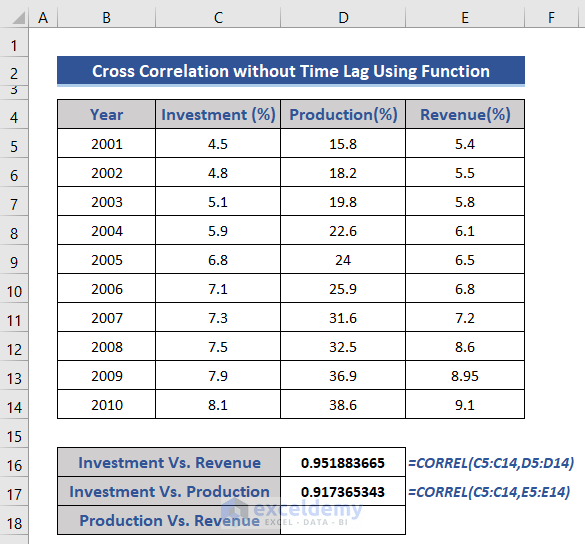
See both cases correlation coefficient is close to 1. This means Production and Revenue are both positively co-related with Investment. Find out the cross-correlation coefficient between Production and Revenue.
- Put the following formula on Cell D18.
=CORREL(D5:D14,E5:E14)
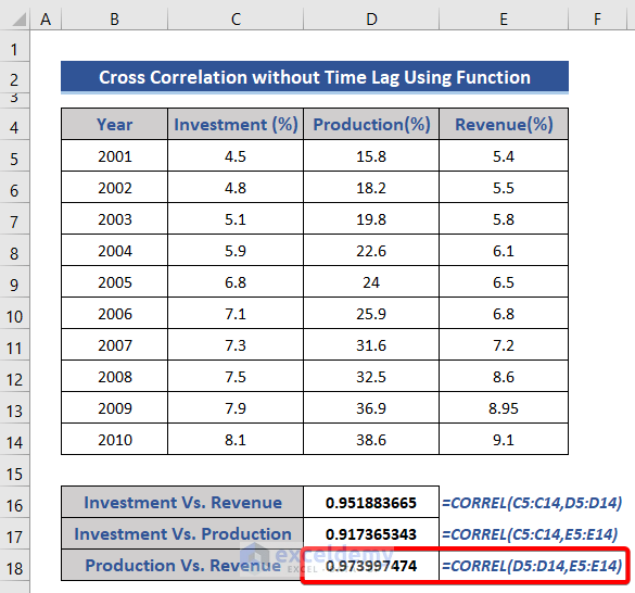
This result is also close to 1. So, Production and Revenue will show similar behavior. If Production increases, Revenue will also increase.
We can also plot the following dataset in a line chart.
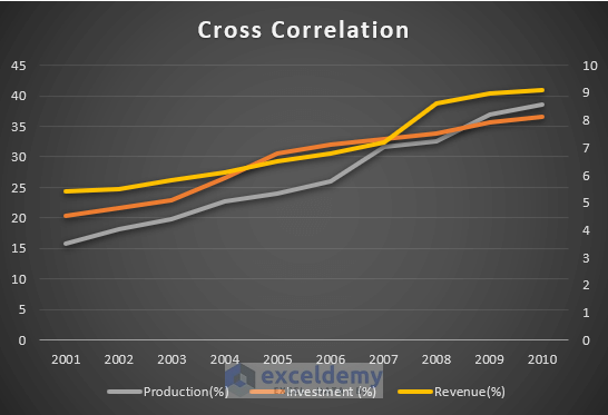
This chart clearly indicates that the other two variables Production and Revenue are positively related to the Investment.
ii. Using the Data Analysis Tool of Analysis-ToolPak
Use default Add-ins of Excel to calculate the cross-correlation.
Steps:
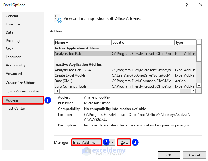
- Go to File >> Options >> Add-ins.
- Select Add-ins and then the Go button.
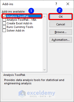
- The Add-ins window appears.
- Choose Analysis Toolpak add-in from the list.
- Press OK.
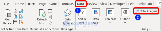
This add-is has been attached to the main tab of Excel.
- Click on the Data Analysis option in the Data tab.
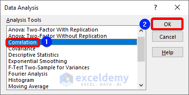
- Select the Correlation option from the Data Analysis window.
- Press the OK button.
- The Correlation window appears.
- Choose the Input Range from the dataset. We choose the Investment, Production, and Revenue columns.
- Tick the Labels in first row option.
- Select a cell as the Output Range.
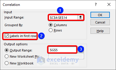
- Click on the OK button.
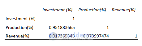
We can see the correlation coefficients are shown here.
Method 2 – Calculate Cross Correlation with Time Lag Using CORREL Function
Steps:
- Calculate the correlative coefficient considering different lags in the Range H5:I9 using the CORREL function.
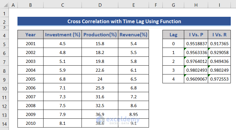
We can see for lag 3; Get the maximum coefficient value.
- Use lag 3 for calculating the cross-correlative coefficient using the following formula.
=CORREL(D5:D11,E8:E14)
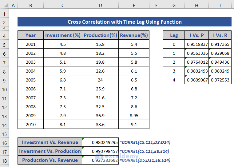
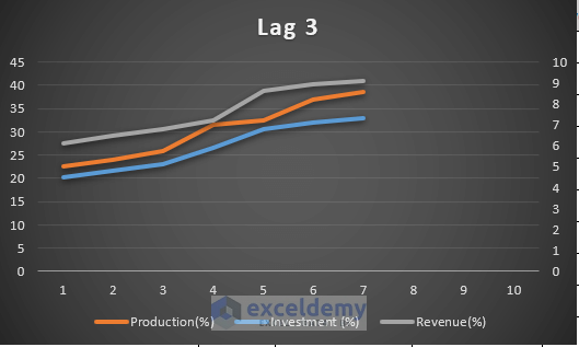
We calculated the cross-correlation for lag 3.
Here is a graph for cross-correlation with time lag 3.
Download Practice Workbook
Download this practice workbook to exercise while you are reading this article.
Related Articles
- How to Make a Correlation Scatter Plot in Excel
- Find Correlation Between Two Variables in Excel
- How to Calculate Correlation between Two Stocks in Excel
- How to Make a Correlation Table in Excel
- How to Make a Correlation Matrix in Excel
- How to Calculate Autocorrelation in Excel
- How to Interpret Correlation Table in Excel
- How to Make Correlation Heatmap in Excel
- How to Do Correlation and Regression Analysis in Excel
<< Go Back to Excel Correlation | Excel for Statistics | Learn Excel
Get FREE Advanced Excel Exercises with Solutions!

this post does not deal with cross-correlation
Hi Don. Thanks for letting us know about this. 🙂 We have updated the blog post. Regards
-ExcelDemy Team