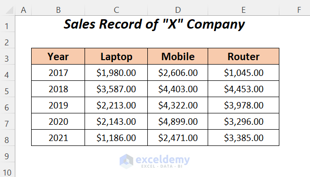
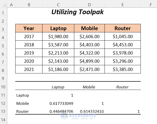
We have the following sample dataset containing sales records of Laptops, Mobile and Routers for different years. We will create a correlation table for demonstrating a relationship between sales values among these products.
Method 1 – Using Analysis Toolpak to Make a Correlation Table in Excel
Steps:
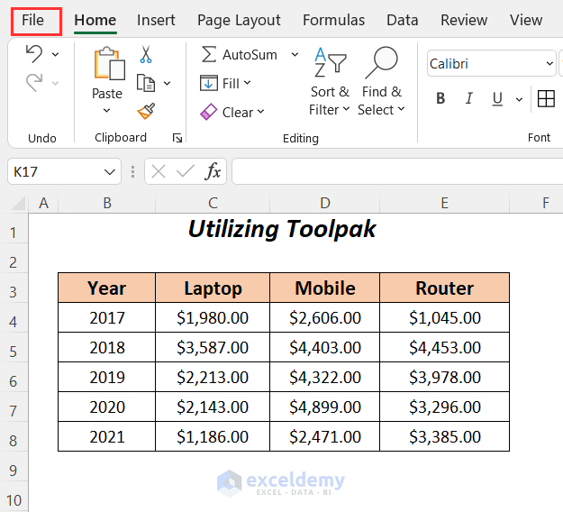
- Go to File.
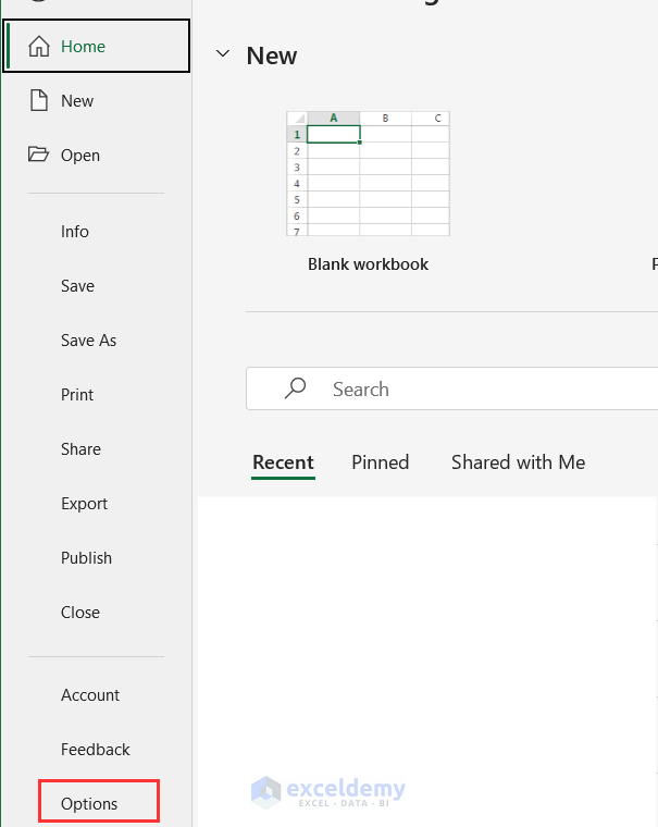
- Select Options.
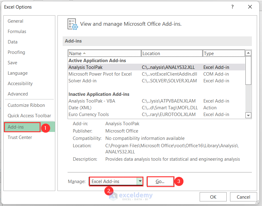
The Excel Options dialog box will open up.
- Click on the Add-ins tab, select Excel Add-ins from Manage options and press Go.
The Add-ins window will pop up.
- Check the Analysis Toolpak option and press OK.
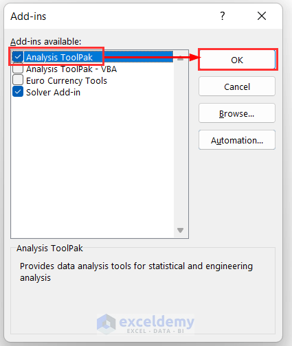
Following this process, you will be able to enable the toolpak.
- Go to the Data tab >> Analyze group >> Data Analysis.
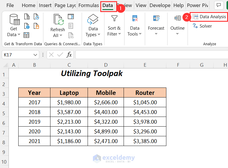
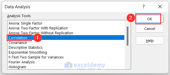
The Data Analysis wizard will pop up.
- Choose the Correlation option and press OK.
- In the Correlation dialog box, select the Input Range as $C$3:$E$8, Output Range as $B$10.
- Choose the option Columns under Grouped By, check Labels in first row option and press OK.
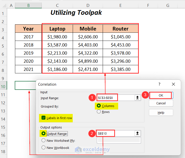
You will get a correlation table below your original dataset.
Read More: How to Make Correlation Heatmap in Excel
Method 2 – Applying CORREL Function to Make a Correlation Table in Excel
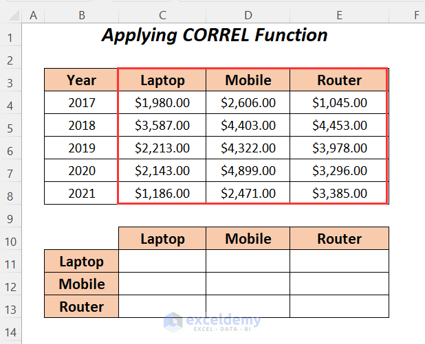
We will be using the CORREL function to create the correlation table for the following sample dataset. We have created a format of this table below the dataset where the names of the products are written as column headers and row headers.
Steps:
- Add the following formula in cell C11.
=CORREL($C$4:$C$8, C$4:C$8)$C$4:$C$8 is the first array that we have referenced absolutely to fix this range for this Laptop row. And C$4:C$8 is the second array which will be fixed by rows but varies with columns.
- Drag the Fill Handle tool to the right.
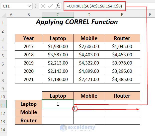
We have completed the first row for the product Laptop.
- For determining relationships between Mobile and the other products, use the following formula.
=CORREL($D$4:$D$8,C$4:C$8)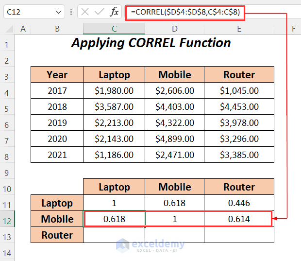
- Use the following formula for the row of the product Router.
=CORREL($E$4:$E$8,C$4:C$8)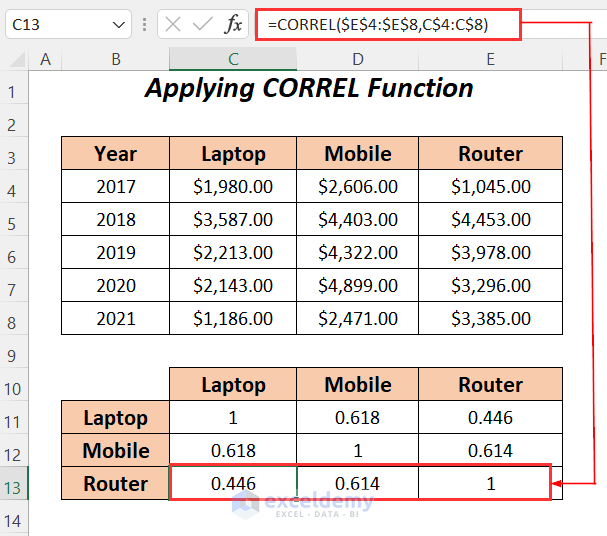
Read More: How to Calculate Autocorrelation in Excel
Method 3 – Use of CORREL and TRANSPOSE Functions
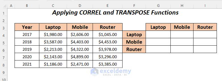
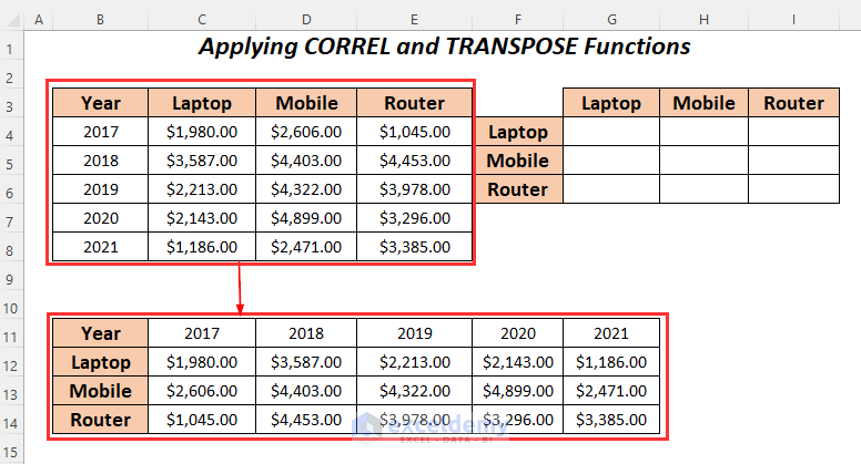
We will use the combination of the TRANSPOSE and CORREL functions to create the correlation table of the products of the following sample dataset.
Steps:
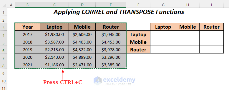
- Press CTRL+C after selecting the dataset to copy it.
- Select the cell where you want to paste (we have selected B11), right-click and choose Transpose from the Paste Options.
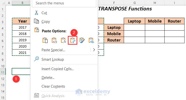
The dataset will be transposed as shown in the following image.
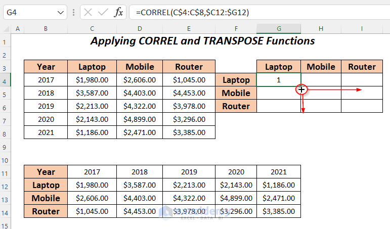
- Add the following formula in cell G4.
=CORREL(C$4:C$8,$C12:$G12)Formula Breakdown
C$4:C$8 → It is the first array from the main dataset, where we have fixed the rows.
$C12:$G12 → This range represents the second array situated in the transposed dataset, where we have fixed the columns.
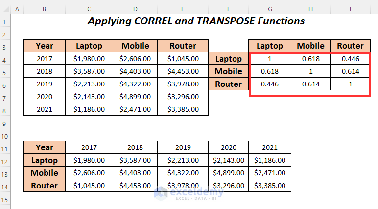
- Drag the Fill Handle tool to the right and down.
The following correlation table will be displayed.
Read More: How to Calculate Partial Correlation in Excel
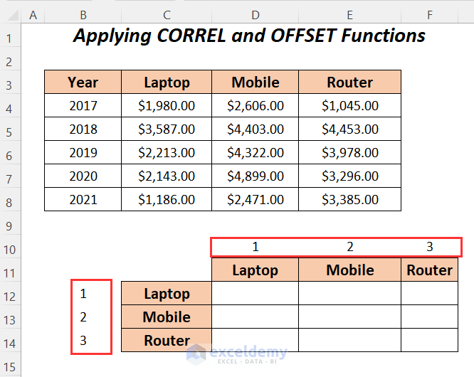
Method 4 – Combination of CORREL and OFFSET Functions to Make a Correlation Table in Excel
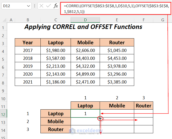
In the table where we will calculate the correlated data, we have listed the serial numbers from 1 to 3 above the column headers and beside the row headers.
Steps:
- Add the following formula in cell D12.
=CORREL(OFFSET($B$3:$E$8,1, D$10,5,1), OFFSET($B$3:$E$8,1,$B12,5,1))Formula Breakdown
OFFSET($B$3:$E$8,1, D$10,5,1) → it is the first array, where $B$3:$E$8 is the main range, 1 is the row number by which the range will go down, D$10 is the column number by which the range will go to the right, 5 is the total row height to be extracted, and 1 is the column number to be extracted.
OFFSET($B$3:$E$8,1,$B12,5,1) → It will extract a range for the second array.
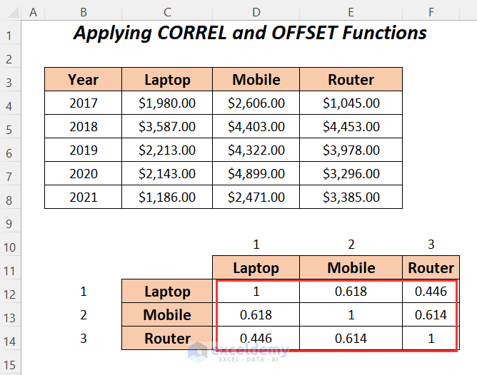
- Drag the Fill Handle tool to the right and down.
The correlation table will be created.
Read More: Find Correlation Between Two Variables in Excel
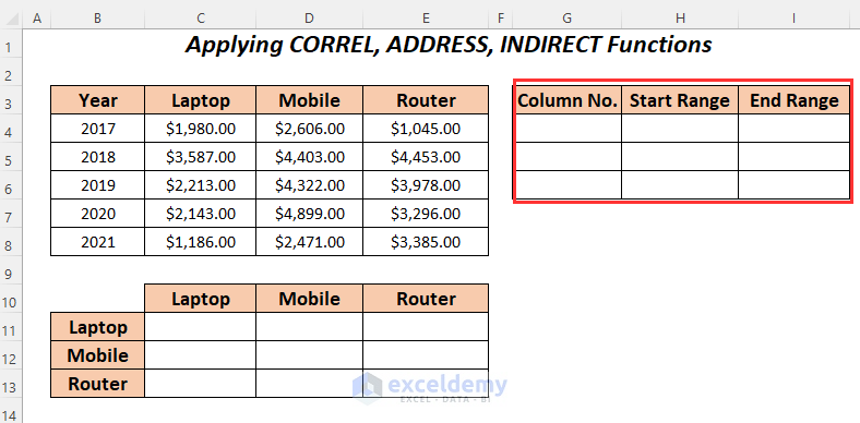
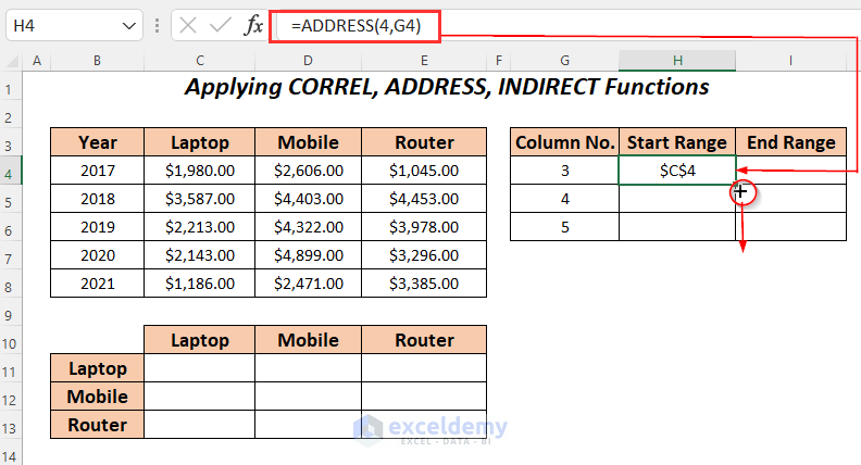
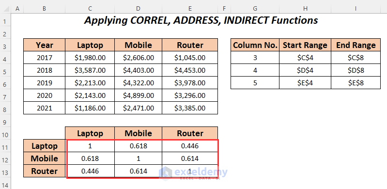
Method 5 – Utilizing ADDRESS and INDIRECT Functions with CORREL Function in Excel
For this method, we have to define the start range and end range of the three columns for the products.
Steps:
- Enter the serial numbers of the columns for the products- Laptop, Mobile and Router.
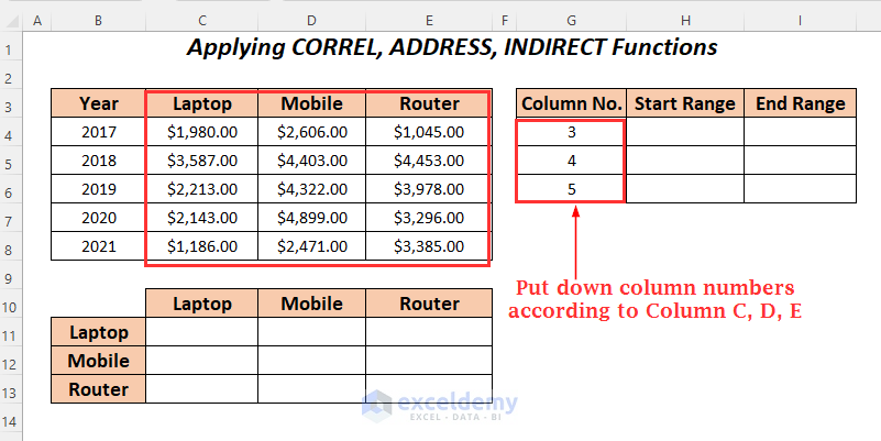
- Add the following formula in cell H4.
=ADDRESS(4, G4)4 is the starting row number with a value in the Laptop column and G4 is the column number.
- Drag down the Fill Handle.
- After having the starting ranges, enter the following formula in cell I4.
=ADDRESS(8, G4)8 is the ending row number with a value in the Laptop column and G4 is the column number.
- Drag down the Fill Handle.
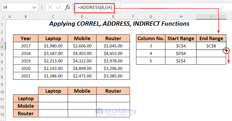
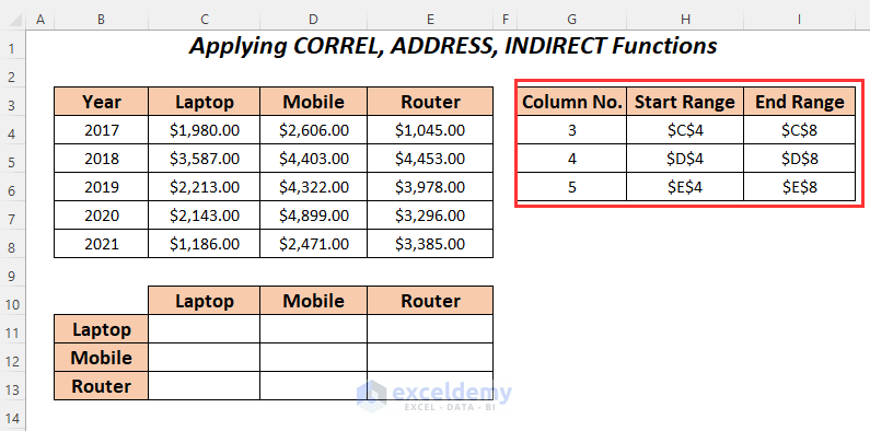
We have completed the ranges.
- Add the following formula in cell C11.
=CORREL(INDIRECT($H4&":"&$I4), C$4:C$8)Formula Breakdown
INDIRECT($H4&”:”&$I4) → it is the first array, where $C$4:$C$8 will be the range.
C$4:C$8 → This range represents the second array where we have fixed the rows.
- Drag the Fill Handle tool to the right and down.
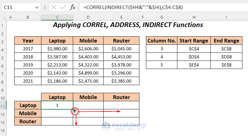
We have created the following correlation table.
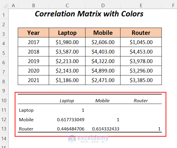
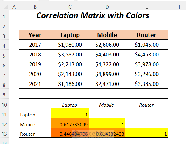
How to Make a Correlation Matrix with Colors in Excel
A correlation matrix is similar to the correlation table created in Method 1. But in this matrix, the cells are colored depending on the ranges.
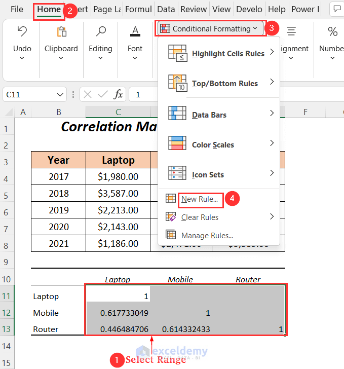
- To highlight the cells of this table, select the range.
- Go to the Home tab >> Conditional Formatting dropdown >> New Rule.
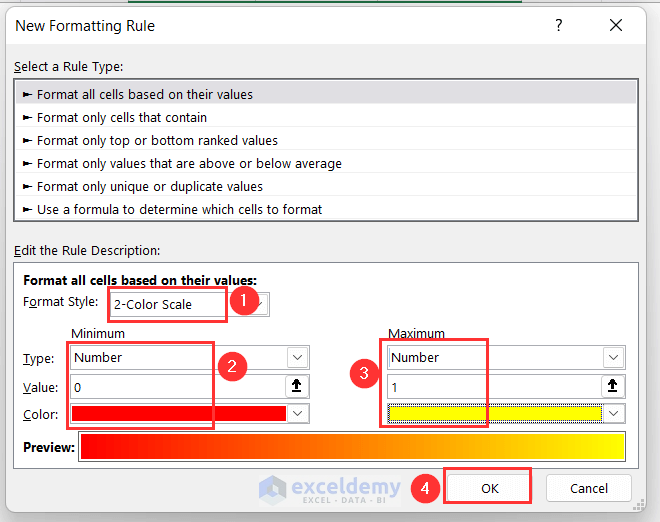
- In the New Formatting Rule dialog box, select the Format all cells based on their values option.
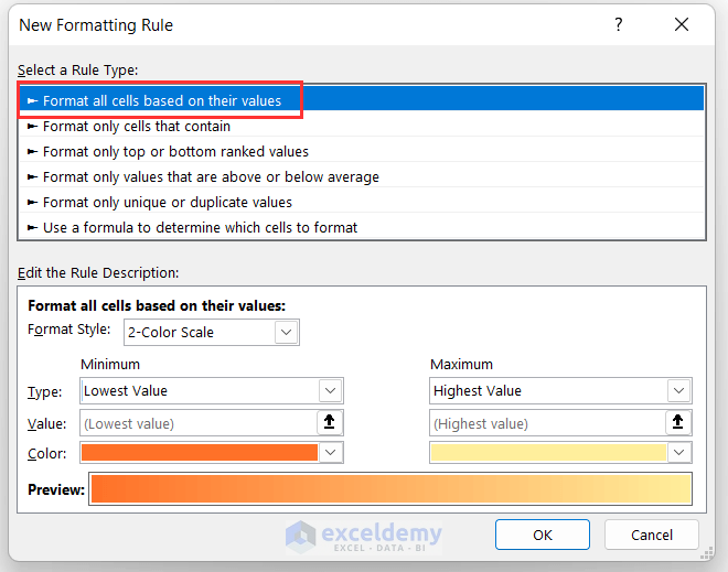
- Choose the Format Style as a 2-Color Scale (because we have a range between 0 and 1).
- Select the following options for Minimum and Maximum values and press OK.
The colors will appear, where Yellow represents 1 and the values between 0 and 1 are represented through the gradient colors.
Download Practice Workbook
Related Articles
- How to Make a Correlation Scatter Plot in Excel
- How to Calculate Cross Correlation in Excel
- How to Calculate Correlation between Two Stocks in Excel
- How to Do Correlation and Regression Analysis in Excel
- How to Interpret Correlation Table in Excel
- How to Make Correlation Graph in Excel
<< Go Back to Excel Correlation | Excel for Statistics | Learn Excel
Get FREE Advanced Excel Exercises with Solutions!
