In this article, we will demonstrate how to make a Correlation Graph in Excel.
Introduction to Correlation Graph in Excel
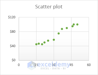
A Correlation Graph is a type of chart which is mostly used in economics, statistics and the social sciences to see the differences or measure relations between two or more variables in a graph.
Direction of Correlation:
There are two types of direction in correlation:
- Positive– When the correlation produces an upward slope, it indicates that the correlation is positive. If variable 1 increases, variable 2 will also increase, and vice versa.
- Negative– When the correlation produces a downward slope, it indicates that the relationship between the variables is inversely proportional, called a negative correlation. If Variable 1 increases, variable 2 will decrease, and vice versa.
Let’s create a Correlation Graph in Excel.
Step 1 – Creating the Correlation Dataset
Suppose we have a dataset of the average temperatures and air conditioners sold in the months of a year.
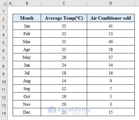
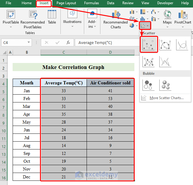
- Select the two columns containing the variables in the dataset.
- Go to “Scatter chart” from the “Insert” tab.
Read More: How to Make Correlation Heatmap in Excel
Step 2 – Inserting and Naming Coordinates to Make the Correlation Graph
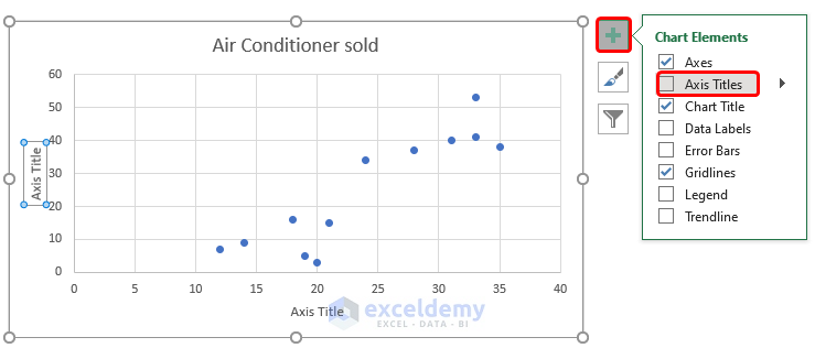
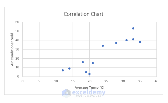
A scatter chart will appear.
- Click on the chart and press on the “plus” sign to open the Options.
- Click “Axis Titles” to name the axes.
After naming the chart, it will look like the following:
Read More: How to Make a Correlation Scatter Plot in Excel
Step 3 – Formatting the Correlation Graph
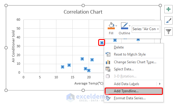
- In the chart, click on any point and right-click on it.
- Choose “Add Trendline”.
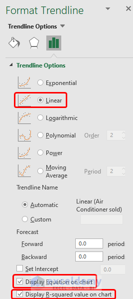
- From the “Format Trendline” option select “Linear”.
- Tick the “Display Equation on Chart” and “Display R-squared value on chart” options.
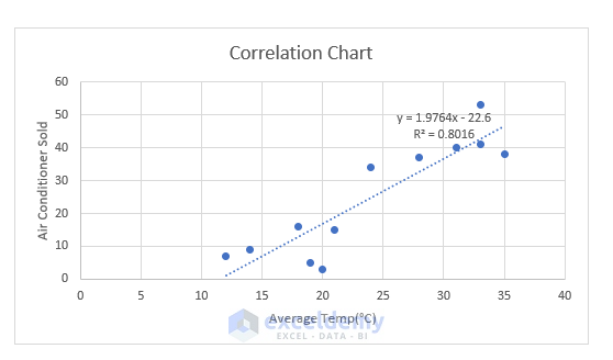
We have successfully created a Correlation Chart in Excel.
Read More: How to Make a Correlation Table in Excel
Things to Remember
- A correlation graph is not able to distinguish between dependent and independent data.
Download Practice Workbook
Related Articles
- How to Calculate Autocorrelation in Excel
- How to Calculate Cross Correlation in Excel
- How to Calculate Correlation between Two Stocks in Excel
- How to Do Correlation and Regression Analysis in Excel
- How to Make a Correlation Matrix in Excel
- How to Interpret Correlation Table in Excel
- How to Calculate Partial Correlation in Excel
<< Go Back to Excel Correlation | Excel for Statistics | Learn Excel
Get FREE Advanced Excel Exercises with Solutions!
