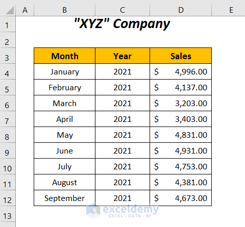
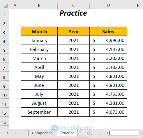
How to Calculate Autocorrelation in Excel (2 Ways)

Here, we have the following dataset containing a company’s sales records over different months. We will try to determine the autocorrelation for different lags in these records between these time ranges using the following 2 methods.

Method 1: Using SUMPRODUCT, OFFSET, AVERAGE, and DEVSQ Functions to Calculate Autocorrelation

Steps:

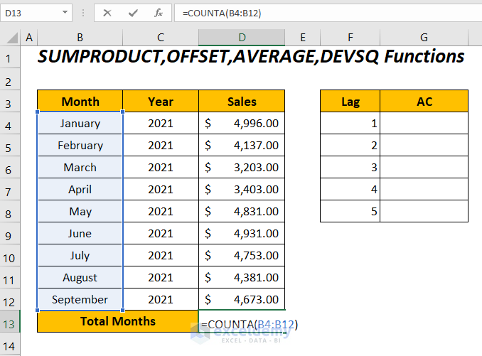
To calculate the total number of months to determine the time series of the sales values.
Enter the following function in cell D13:

=COUNTA(B4:B12)

COUNTA will determine the total months in the range B4:B12.

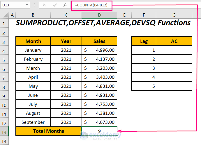
Press ENTER to get the total number of months: 9.

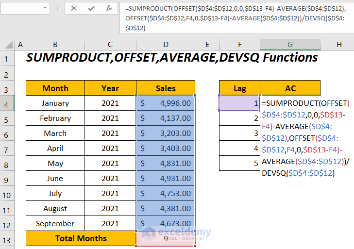
To determine the autocorrelations for the sales series between the lags 1 to 5.
Enter the following formula in cell G4:

=SUMPRODUCT(OFFSET($D$4:$D$12,0,0,$D$13-F4)-AVERAGE($D$4:$D$12),OFFSET($D$4:$D$12,F4,0,$D$13-F4)-AVERAGE($D$4:$D$12))/DEVSQ($D$4:$D$12)

Here, $D$4:$D$12 is the Sales range, $D$13 is the total number of months, and F4 is the lag value.

$D$13-F4 becomes
9-1 → 8

OFFSET($D$4:$D$12,0,0,$D$13-F4) becomes
OFFSET($D$4:$D$12,0,0,8) → extracts a range with a height of 8 rows from the reference cell $D$4.
Output → {4996; 4137; 3203; 3403; 4831; 4931; 4753; 4381}

AVERAGE($D$4:$D$12) → determines the average value of this range
Output → 4367.555

OFFSET($D$4:$D$12,0,0,$D$13-F4)-AVERAGE($D$4:$D$12) becomes
{4996; 4137; 3203; 3403; 4831; 4931; 4753; 4381}-4367.555
Output → {628.444; -230.556; -1164.556; -964.556; 463.444; 563.444; 385.444; 13.444}

OFFSET($D$4:$D$12,F4,0,$D$13-F4) becomes
OFFSET($D$4:$D$12,1,0,8) → the starting cell reference moves 1 cell downwards from $D$4 and then extracts a range with a height of 8 rows from the reference cell $D$5
Output → {4137; 3203; 3403; 4831; 4931; 4753; 4381; 4673}

OFFSET($D$4:$D$12,F4,0,$D$13-F4)-AVERAGE($D$4:$D$12) becomes
{4137; 3203; 3403; 4831; 4931; 4753; 4381; 4673}-4367.555
Output → { -230.556; -1164.556; -964.556; 463.444; 563.444; 385.444; 13.444; 305.444}

SUMPRODUCT(OFFSET($D$4:$D$12,0,0,$D$13-F4)-AVERAGE($D$4:$D$12),OFFSET($D$4:$D$12,F4,0,$D$13-F4)-AVERAGE($D$4:$D$12)) becomes
SUMPRODUCT({628.444; -230.556; -1164.556; -964.556; 463.444; 563.444; 385.444; 13.444},{ -230.556; -1164.556; -964.556; 463.444; 563.444; 385.444; 13.444; 305.444})
Output → 1287454.358

DEVSQ($D$4:$D$12) → returns the sum of squares of the deviations of the data range from their mean.
Output → 3508950.222

SUMPRODUCT(OFFSET($D$4:$D$12,0,0,$D$13-F4)-AVERAGE($D$4:$D$12),OFFSET($D$4:$D$12,F4,0,$D$13-F4)-AVERAGE($D$4:$D$12))/DEVSQ($D$4:$D$12) becomes
1287454.358/3508950.222
Output → 0.366905848

Press ENTER and drag down the Fill Handle tool.

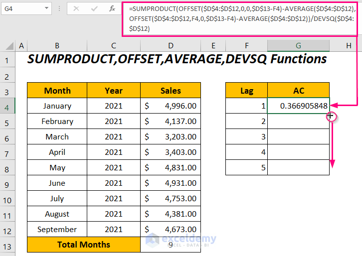
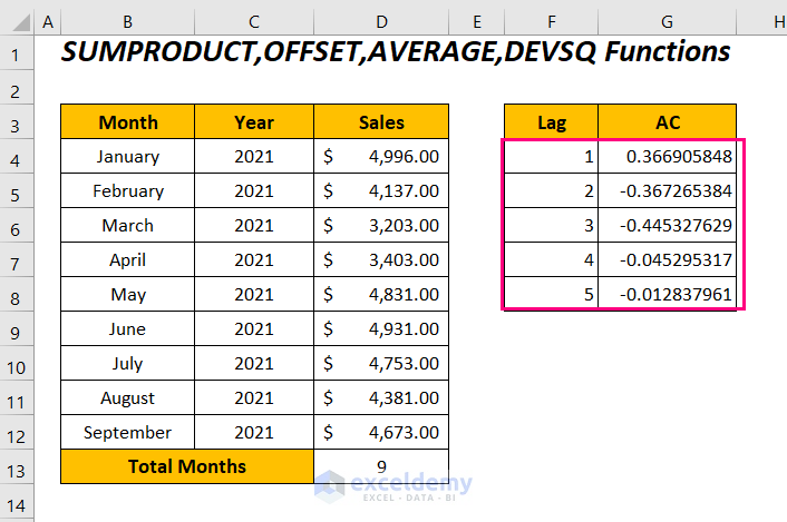
You will get the autocorrelations for the monthly sales series between a range of lags from 1 to 5.

Method 2 – Using SUMPRODUCT, AVERAGE, VAR.P Functions to Calculate Autocorrelation in Excel

Steps:

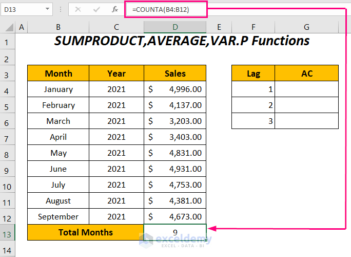
Enter the following function in cell D13 to determine the total number of rows in the data series:

=COUNTA(B4:B12)

COUNTA will determine the total months in the range B4:B12.

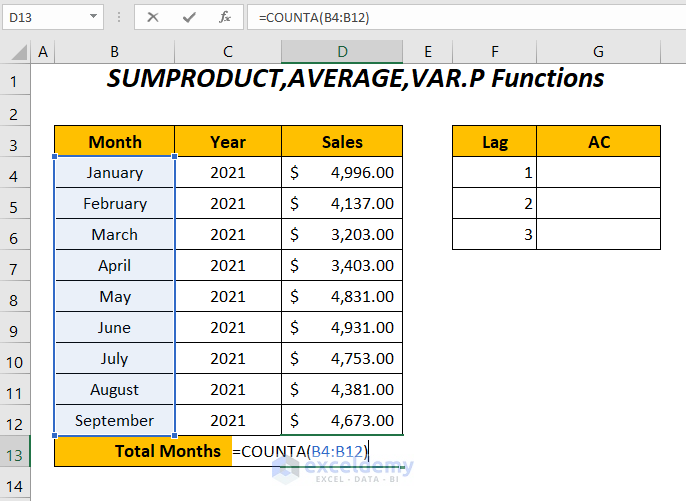
Press ENTER to get the total number of months: 9.

To determine the autocorrelations for the sales series between the lags 1 to 3.
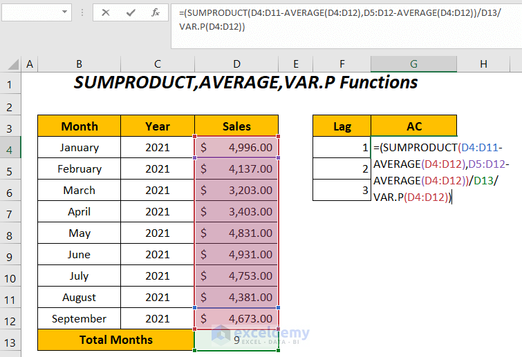
Enter the following formula in cell G4:

=(SUMPRODUCT(D4:D11-AVERAGE(D4:D12),D5:D12-AVERAGE(D4:D12))/D13/VAR.P(D4:D12))

Here, D4:D11 is the Sales range without the last cell value due to lag 1, similarly, D5:D12 is the Sales range without the first cell value due to lag 1, and D13 is the total number of months.

AVERAGE(D4:D12) → determines the average value of this range
Output → 4367.555

D4:D11-AVERAGE(D4:D12) becomes
{4996; 4137; 3203; 3403; 4831; 4931; 4753; 4381}-4367.555
Output → {628.444; -230.556; -1164.556; -964.556; 463.444; 563.444; 385.444; 13.444}

D5:D12-AVERAGE(D4:D12) becomes
{4137; 3203; 3403; 4831; 4931; 4753; 4381; 4673}-4367.555
Output → { -230.556; -1164.556; -964.556; 463.444; 563.444; 385.444; 13.444; 305.444}

SUMPRODUCT(D4:D11-AVERAGE(D4:D12),D5:D12-AVERAGE(D4:D12)) becomes
SUMPRODUCT({628.444; -230.556; -1164.556; -964.556; 463.444; 563.444; 385.444; 13.444},{ -230.556; -1164.556; -964.556; 463.444; 563.444; 385.444; 13.444; 305.444})
Output → 1287454.358

SUMPRODUCT(D4:D11-AVERAGE(D4:D12),D5:D12-AVERAGE(D4:D12))/D13 becomes
1287454.358/9
Output → 143050.484224966

P(D4:D12) → determines variance based on the entire range.
Output → 389883.358024691

(SUMPRODUCT(D4:D11-AVERAGE(D4:D12),D5:D12-AVERAGE(D4:D12))/D13/VAR.P(D4:D12)) becomes
(143050.484224966/389883.358024691)
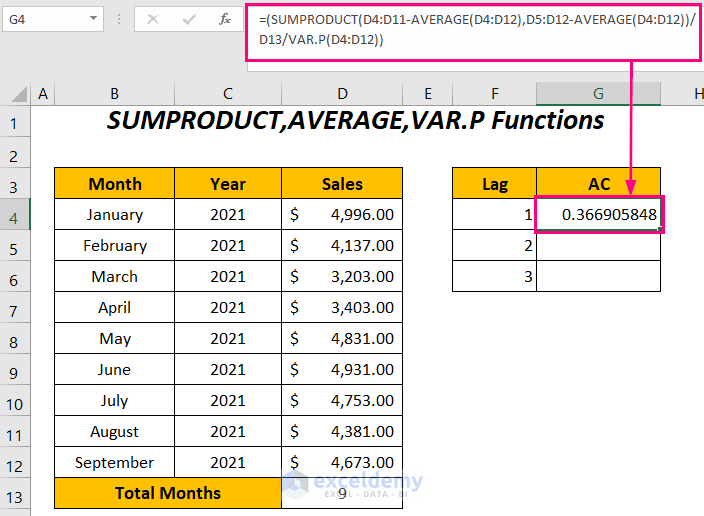
Output → 0.366905848

Press ENTER.
You will get the autocorrelation of the sales series with their one-lagged version.

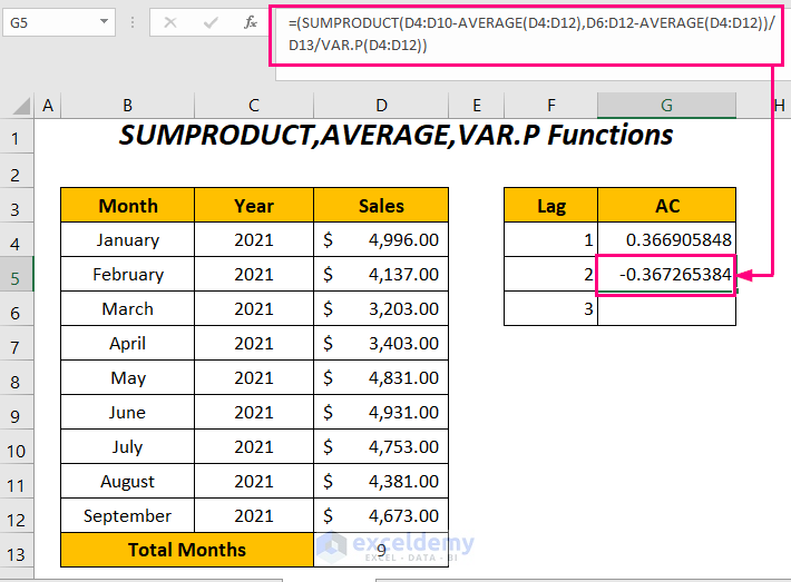
To get the autocorrelation for lag=2, enter the following formula:

=(SUMPRODUCT(D4:D10-AVERAGE(D4:D12),D6:D12-AVERAGE(D4:D12))/D13/VAR.P(D4:D12))

D4:D10 represents the sales series without the last two values due to lag 2 and D6:D12 is the series without the first two values.

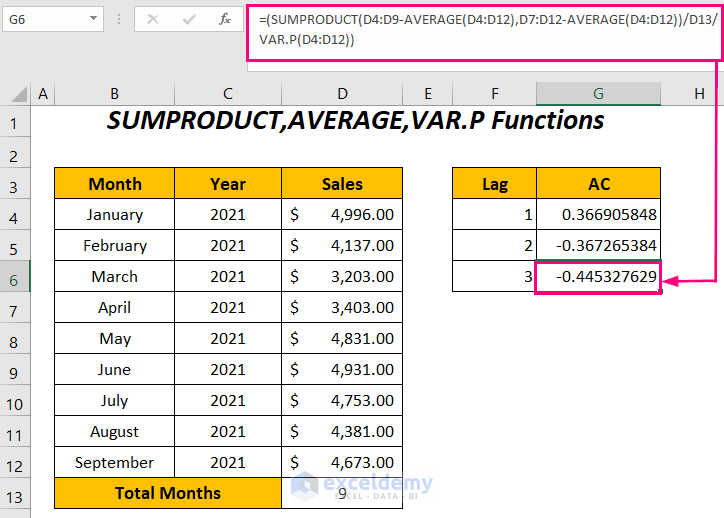
You can have the autocorrelation for lag=3 by entering the following formula:

=(SUMPRODUCT(D4:D9-AVERAGE(D4:D12),D7:D12-AVERAGE(D4:D12))/D13/VAR.P(D4:D12))

D4:D9 represents the sales series without the last three values due to lag 3 and D7:D12 is the series without the first three values.

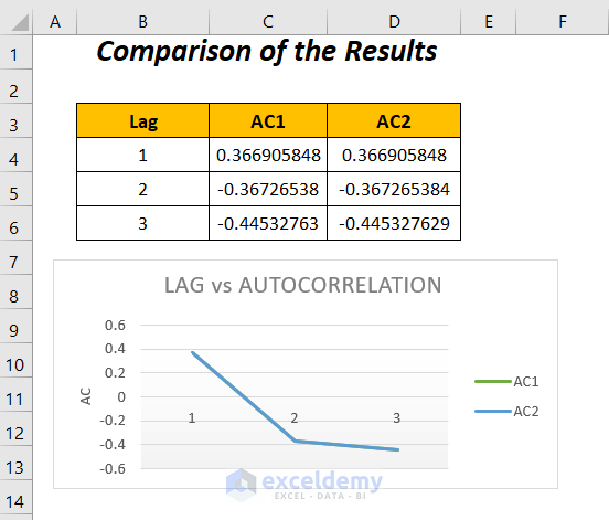
Comparison of Results with Graphical Representation

We get the same autocorrelation values for their corresponding lags by using the above two formulas in two methods. Moreover, it can be concluded that with the increasing lagged values, we are experiencing a series of decreased autocorrelations.
For the lag value 1, we have a positive value which represents a proportionate increase in this time interval. And, for the rest of the lag values, we have negative autocorrelations defining a proportionate decrease in the time intervals.

Practice Section

Download the Workbook

Autocorrelation Calculation.xlsx

<< Go Back to Excel Correlation | Excel for Statistics | Learn Excel

Get FREE Advanced Excel Exercises with Solutions!

2 Comments

Allen Hartman Jan 4, 2024 at 1:41 AM

Hi,

Interesting article. Thank you for sharing, but I am still confused about how to apply what you have shared in my application.

I have digitized vibration sensor data from rotating machinery. My set of values that I paste into the Excel column is 1808 cells long. This is the number of samples that are acquired in a single rotation of the shaft.

I am not an expert in Excel, or statistics. My understanding is that Autocorrelation should always result in values between +1 and -1. I would like to have an output that I can plot in a x-y line chart or better yet in a “chart” that represents one shaft rotation (for visualization purposes).

I do not know how many (lag) segments to use but once I understand how to properly configure this I could experiment with lag to find what might be appropriate.

Do you have a recommendation for how I should approach this?
- Reply
  Yousuf Khan Jan 17, 2024 at 12:00 AM
  Hello Allen,
  Thank you for sharing your experience with us. I understand you want to know how the lag segments work to properly configure your digitized vibration sensor data from rotating machinery.
  Here are factors to consider:
  1. Longer data means you can use more lag values without losing reliability.
  2. More frequent data collection might need more lag values to find detailed patterns.
  3. If you expect specific patterns, use enough lag values to catch them.
  4. To detect repeating patterns, use enough lags to cover potential periods.
  5. More lags require more calculations, potentially slowing processing. Balance accuracy and efficiency based on available resources.
  6. With your data resolution, you could start with around 40-50 lags to capture potential patterns within a rotation.
  7. Finally, there’s no universally optimal lag length. It depends on your data, analysis objectives, and computational constraints.
  
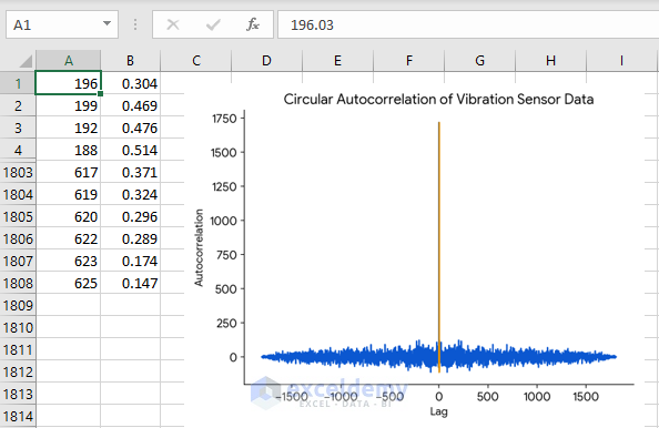
  Let’s calculate the autocorrelation with a data range similar to yours using a different technique. Since you have significantly large data, you can consider this method. I am going to calculate autocorrelation using Excel VBA to make the process faster and more accurate. Follow the steps:
  1. Line up your data.
  2. Run the below VBA code:
```
Sub CalculateAutocorrelation()
'Developed by ExcelDemy
    Dim dataRange As Range
    Set dataRange = Range("A1:A1808")
    Dim autocorrelationValues As Variant
    ReDim autocorrelationValues(1 To dataRange.Cells.Count)

    For i = 1 To dataRange.Cells.Count
        autocorrelationValues(i) = CalculateAutocorrelationForLag(dataRange, i - 1)
    Next i
    Range("B1").Resize(UBound(autocorrelationValues), 1).Value = autocorrelationValues
    ActiveSheet.Shapes.AddChart.Select
    ActiveChart.ChartType = xlXYScatter
    ActiveChart.SetSourceData Source:=Range("A1:B1808")
End Sub

Function CalculateAutocorrelationForLag(dataRange As Range, lag As Integer) As Double
    Dim mean As Double
    Dim numerator As Double
    Dim denominator As Double
    mean = Application.WorksheetFunction.Average(dataRange)
    For i = 1 To dataRange.Cells.Count - lag
        numerator = numerator + (dataRange.Cells(i) - mean) * (dataRange.Cells(i + lag) - mean)
        denominator = denominator + (dataRange.Cells(i) - mean) ^ 2
    Next i
    CalculateAutocorrelationForLag = numerator / denominator
End Function 
```
  As a result, you will obtain the scatter chart visualizing your output.
  
  You can use the effective methods mentioned in the article too. Hope this helps!
  
  Regards,
  Yousuf Khan Shovon

How to Calculate Autocorrelation in Excel (2 Ways)

Method 1: Using SUMPRODUCT, OFFSET, AVERAGE, and DEVSQ Functions to Calculate Autocorrelation

Method 2 – Using SUMPRODUCT, AVERAGE, VAR.P Functions to Calculate Autocorrelation in Excel

Comparison of Results with Graphical Representation

Practice Section

Related Articles

Leave a reply Cancel reply