What Is the Spearman Correlation?
The Spearman Correlation is a derivative of the Pearson Correlation Coefficient in nonparametric form.
This value determines the linear correlation between two sets of data, often denoted by rs or ⲣ.
The Pearson Product Moment Correlation determines the linear relationship between continuous variables. The general expression of Pearson Correlation is:

RX and RY are the values that are ranked and the standard deviation of the datasets.
The Spearman Correlation evaluates the monotonic relationship between the values.
The complete form of the Spearman Coefficient is
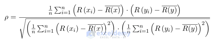
This version is a slightly modified version of Pearson’s equation. Here,
- Rx and Ry denote the rank of the x and y variables.
- R̅(x) and R̅(Y) are the mean ranks.
Use the Spearman correlation:
- If your data has outliers that can influence the result.
- If the data is in a non-linear relationship or not fully distributed.
- If one of the variables is ordinal.
The range of the Spearman Correlation coefficient value ranges from +1 to 1.
- 1 indicates a perfect correlation. Both datasets are matched.
- -1 indicates negative correlated data.
- 0 shows no correlation between data.
The sample dataset showcases two arrays.

Method 1 – Using an Excel Formula to Calculate the Spearman Correlation
A simple approximation to the Spearman Correlation is the following:
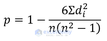
di is the difference between a pair of ranks
And n is the number of observations.
This formulation won’t work if there is tied value in ranking.
Steps
- To rank the value of the columns Math and Economics, enter the following formula in E5 and press enter:
=RANK.AVG(C5,$C$5:$C$14,0)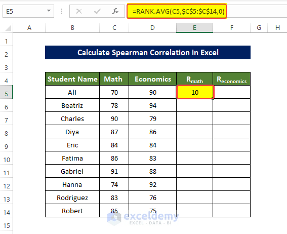
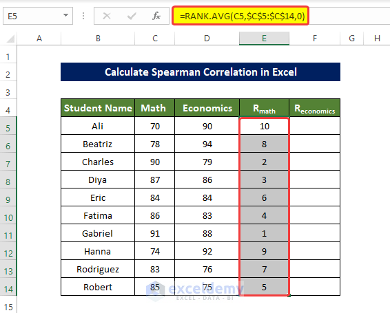
- Drag down the Fill Handle to see the result in the rest of the cells.
The values in E5:E14 are ranked.
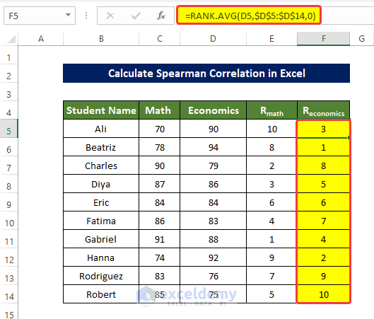
- To rank D5:D14, enter the following formula in F5 and press enter:
=RANK.AVG(D5,$D$5:$D$14,0)
- Drag down the Fill Handle to see the result in the rest of the cells.
The values in F5:F14 are ranked.
The ranks of both Math and Economics column values does not contain any tied value, there is no value with the same rank.
To calculate the Spearman correlation in the Excel worksheet:

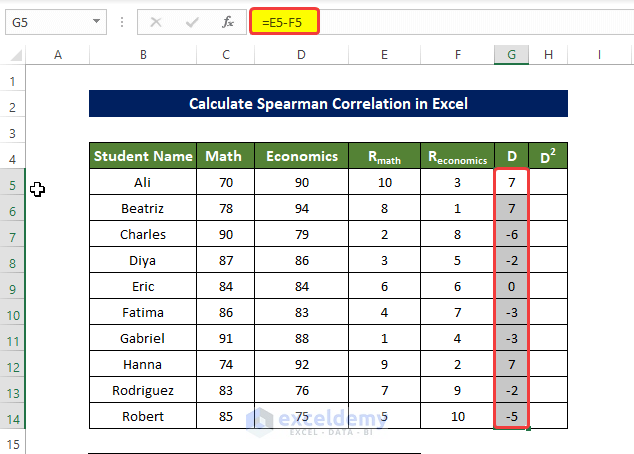
- Find the difference between the ranked value in each row.
- Enter the following formula in G5 and press enter:
=E5-F5 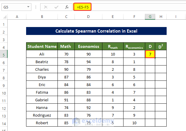
- Drag down the Fill Handle to see the result in the rest of the cells.
The difference between the ranked values in each row is displayed in G5:G14.
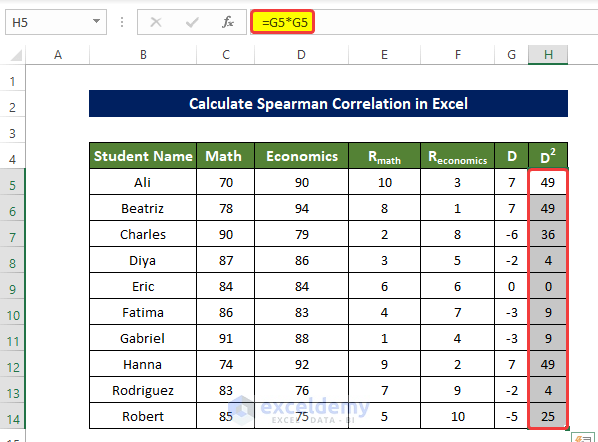
- To find the square of the difference between the ranked value in each row, calculated in D5:D14, enter the following formula in H5 and press enter:
=G5*G5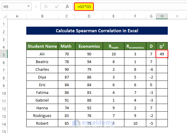
- Drag down the Fill Handle to see the result in the rest of the cells.
The square of the difference between all ranked values in each row is displayed in H5:H14.
- To get the sum of H5:H15, enter the following formula in H15:
=SUM(H5:H14)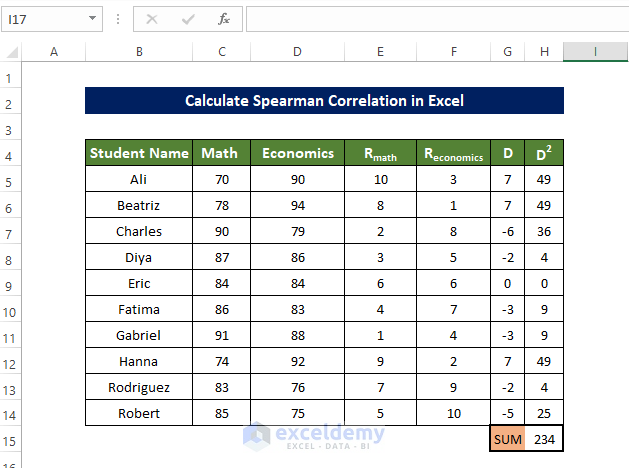
- Enter the number of entries in E16, here, 10.
- Enter the following formula in E17:
=1-(6*H15)/(E16^3-E16)You will get the Spearman Correlation.
The output is a negative value, which indicates a negative correlation between the two ranked data columns.
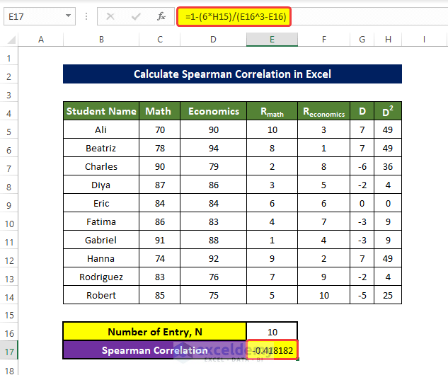
If the value of one column increases, the value in the other column will not increase, and vice versa.
Read More: How to Find Spearman Rank Correlation Coefficient in Excel
Method 2 – Inserting the CORREL Function to Compute the Spearman Correlation
Steps
- To rank the value of the columns Math and Economics, enter the following formula in E5 and press enter:
=RANK.AVG(C5,$C$5:$C$14,0)
- Drag down the Fill Handle to see the result in the rest of the cells.
The values in E5:E14 are ranked.

- To rank the range F5:F14, enter the following formula in F5 and press enter:
=RANK.AVG(D5,$D$5:$D$14,0)
- Drag down the Fill Handle to see the result in the rest of the cells.
The values in F5:F14 are ranked.

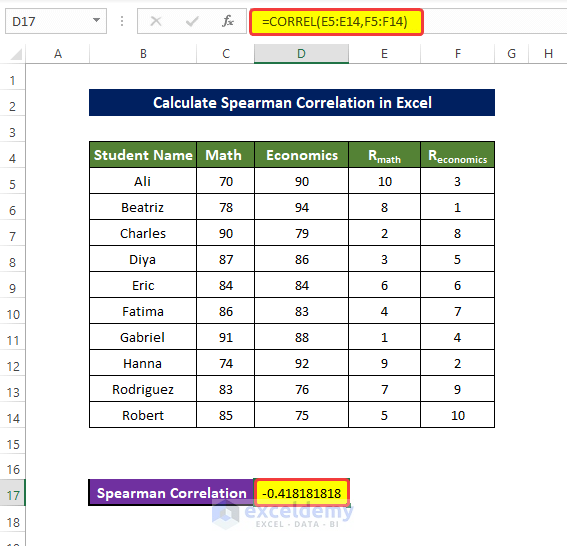
- Select D17 and enter the following formula:
=CORREL(E5:E14,F5:F14)
The Spearman correlation is displayed in D17.
Read More: How to Calculate P Value for Spearman Correlation in Excel
Method 3 – Calculating the Spearman Correlation Using a Graph in Excel
Steps
- To rank the value of the columns Math and Economics, enter the following formula in E5 and press enter:
=RANK.AVG(C5,$C$5:$C$14,0)
- Drag down the Fill Handle to see the result in the rest of the cells.
The values in E5:E14 are ranked.

- To rank F5:F14, enter the following formula in F5 and press enter:
=RANK.AVG(D5,$D$5:$D$14,0)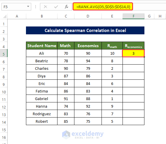
- Drag down the Fill Handle to see the result in the rest of the cells.
The values in F5:F14 are ranked.
- Create a scatter plot with the ranked columns: select both RMath and REconomics.
- In the Insert tab, go to Scatter in Charts and click Scatter plot.
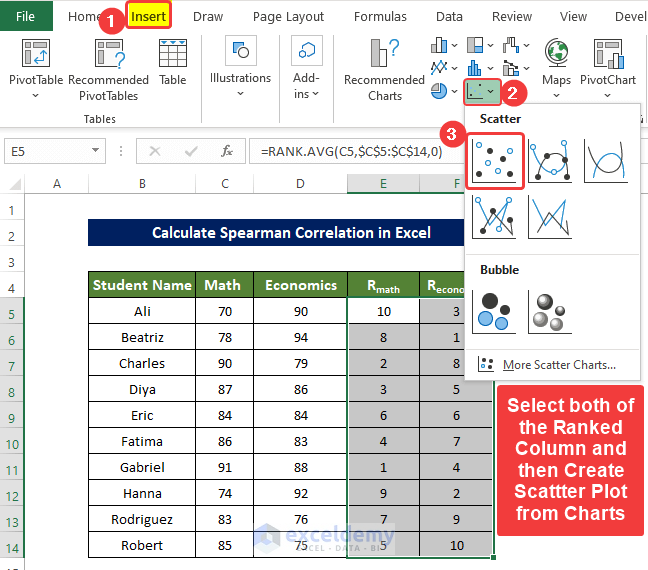
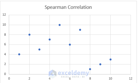
- The chart will display the RMath column values in the X-axis and the REconomics values in the Y-axis.
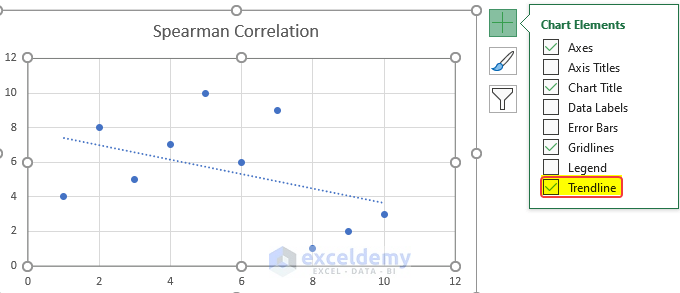
- Click Chart Elements.
- Check Trendline.
- A downward-facing Trendline will be displayed in the chart.
- Double-click the chart.
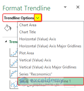
- In the new window, click Trendline options.
- Select the Trendline you created.
- Click the histogram-shaped icon.
- Check Display R squared value on chart.
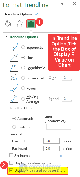
- The R-value is displayed.
- Note it down.
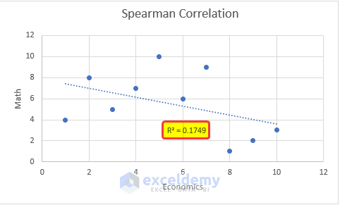
- Select E16 and enter the value of R2.
- To square root the R2 value and get the value of Spearman Correlation, enter the following formula in E18:
=SQRT(E16)- Mind the slope of the trendline: if it is downward, alter the sign in E18. If the slope is upward, no change is needed. Here, the trendline is downward. The sign in E18 is changed from 0.41821 to -0.4821.
This is the final value of the Spearman Correlation.
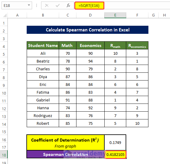
The negative value shows a negative correlation between the data columns.
Read More: How to Find Correlation Coefficient in Excel Scatter Plot
Download Practice Workbook
Download the practice workbook.
Related Articles
- How to Show Relationship Between Two Variables in Excel Graph
- How to Calculate Correlation Coefficient in Excel
- How to Find Coefficient of Determination in Excel
- How to Calculate Intraclass Correlation Coefficient in Excel
<< Go Back to Excel Correlation | Excel for Statistics | Learn Excel
Get FREE Advanced Excel Exercises with Solutions!

Thanks for the tutorial. my question is how i can find or calculate the critical values to assess its significance?
Thanks for your question. Actually, you can approach this problem in two separate ways. One is directly calculating the significant value or using a chart. For the chart, you need to calculate the T value first, and then you will calculate the p-value. Using them, you can calculate the critical value from a chart available online.
1. The formula for calculating the T value is, t=r_s×√((n-2)/(1-r_s^2 ))
Where r_s is the Spearman correlation value.
n is the no of entry
The Excel formula would be in our case =E17*SQRT((E16-2)/(1-E17^2))
2. The formula for significant value, p =T.DIST.2T(ABS(calculated t value),n-2)
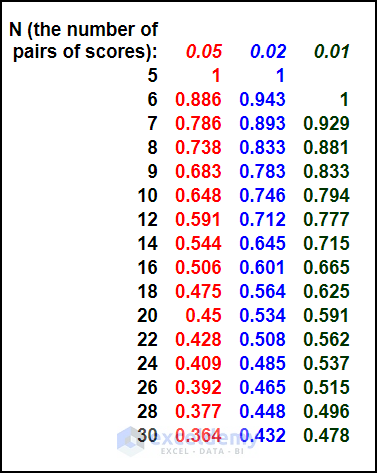
3. To calculate the critical value, you need to have a critical value chart. Using the p-value and the n (Number of entries), from the chart, you need to get the critical value.
4. You may be needed to interpolate the critical values as you may not have the exact p or n values. If your correlation value>critical value, then there is a significant correlation between the values. In other words, the correlation result is significant.