In Excel, the CORREL function is used to determine how closely two sets of data are associated with each other. In this article, we will show you how to use the CORREL function in Excel.
Introduction to the CORREL Function
- Description
The CORREL function is a Statistical function in Excel. It calculates the correlation coefficient of two cell ranges. For example, you can calculate the correlation between two stock markets, between height-weight measurements, between exam results of two semesters, etc.
- Syntax
=CORREL(array1, array2)
- Arguments Description
| Argument | Required/ Optional | Description |
|---|---|---|
| array1 | Required | A range of cell values. |
| array2 | Required | The second range of cell values. |
- Equation
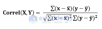
Here,
![]()
means the Average of array1 and array2 respectively.
- Return Value
The correlation coefficient – a value between -1 and +1 – of two sets of variables.
CORREL Function in Excel: 3 Methods
In this section, we will show you the basic method of how to utilize the CORREL function in Excel. We will also discuss the Perfect Positive and Negative Correlation between two arrays with the CORREL function.
1. Generic Example of the CORREL Function
We will show you how to implement the CORREL function with an example of calculating the correlation coefficient between Age and Weight. You can also implement these same steps to find out the correlation coefficient between stock markets, results, height-weight measurements, etc.
Steps to calculate the correlation coefficient between Age and Weight are given below.
Steps:
- Pick a cell to store the result (in our case, it is cell C15).
- Write the CORREL function and pass the array values or cell ranges inside the parentheses.
In our case, the formula was,
=CORREL(B5:B13, C5:C13)Here,
B5:B13 = array1, the first range of cells, column Age
C5:C13 = array2, the second range of cells, column Weight
- Press Enter.
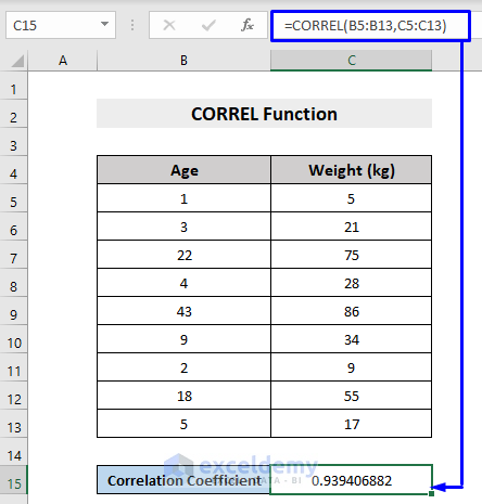
You will get the correlation coefficient between the range of values defined in your dataset.
2. CORREL Function with Perfect Positive Correlation
Perfect Positive Correlation means a correlation coefficient of “+1”. In Perfect Positive Correlation, when variable X increases, variable Y increases along with it. When variable X decreases, variable Y decreases too.
Look at the following example to understand more.
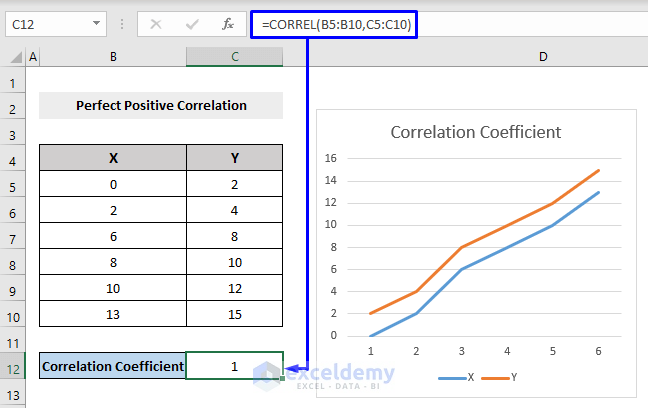
Here X and Y axes, both have seen an upward trend therefore it is a Perfect Positive Correlation, producing result 1.
3. CORREL Function with Perfect Negative Correlation
Perfect Negative Correlation means a correlation coefficient of “-1”. In Perfect Negative Correlation, when variable X increases, variable Y decreases, and when variable X decreases variable Y increases.
Look at the following example.
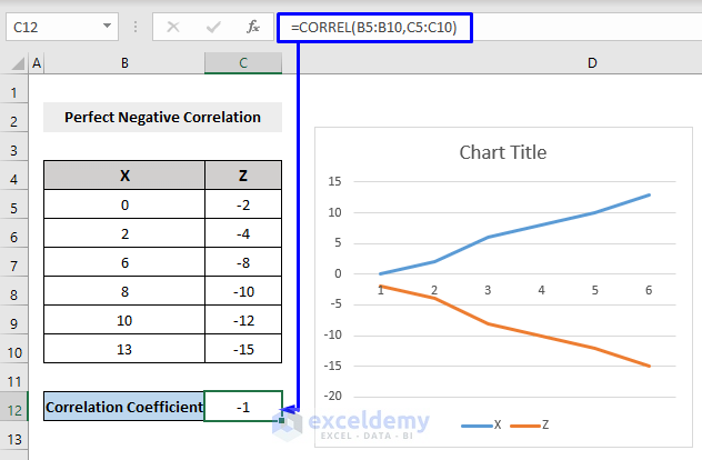
Here X-axis has witnessed a steady growth while the Z-axis has experienced a downward trend, therefore it is a Perfect Negative Correlation with the result of “-1”.
Insert CORREL Function from Excel Command Tool
You can also insert the CORREL function from Excel’s command tool and extract the correlation coefficient between data from there.
Steps to calculate the correlation coefficient between arrays (Height Column and Weight Column) from Excel’s command tool are shown below.
Steps:
- Pick a cell to store the result (in our case, it is cell C15).
- Next, go to Formulas -> More Functions -> Statistical -> CORREL
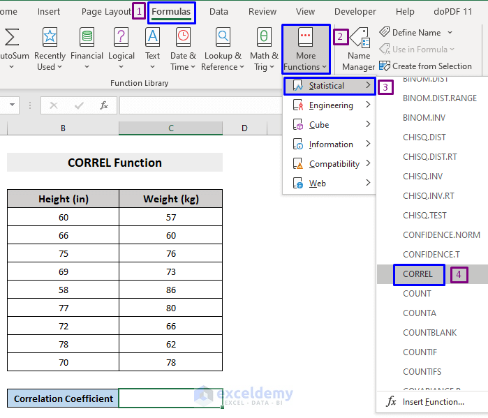
- In the Function Arguments pop-up box, select the Array1 by dragging through the whole 1st column or row and the Array2 by dragging through the whole 2nd column or row of your dataset.
In our case,
Array1 = B5:B13, the Height Column
Array2 = C5:C13, the Weight Column

- Press OK.

In this way too, you will get the correlation coefficient between two arrays of your dataset.
CORREL Function in VBA
The CORREL function can also be used with VBA in Excel. The steps to do that are shown below.
Steps:
- Press Alt + F11 on your keyboard or go to the tab Developer -> Visual Basic to open Visual Basic Editor.

- In the pop-up code window, from the menu bar, click Insert -> Module.

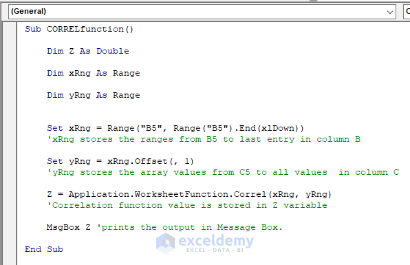
- Copy the following code and paste it into the code window.
Sub CORRELfunction()
    Dim Z As Double
    Dim xRng As Range
    Dim yRng As Range
    Set xRng = Range("B5", Range("B5").End(xlDown)) 'xRng stores the ranges from B5 to last entry in column B
    Set yRng = xRng.Offset(, 1) 'yRng stores the array values from C5 to all values  in column C
    Z = Application.WorksheetFunction.Correl(xRng, yRng) 'Correlation function value is stored in Z variable
    MsgBox Z 'prints the output in Message Box.
End Sub
Your code is now ready to run.
- Press F5 on your keyboard or from the menu bar select Run -> Run Sub/UserForm. You can also just click on the small Play icon in the sub-menu bar to run the macro.

You will get a Microsoft Excel pop-up message box showing the correlation coefficient result between two cell ranges of your dataset.

Things to Remember
- If an array or cell range contains text, logical values, or blank cells, those values are ignored. However, cells with zero are counted as arguments.
- #N/A error will be returned if array1 and array2 have different numbers of data points.
- #DIV/0! error will occur if either array1 or array2 is empty, or if the Standard Deviation (S) of their values is equal to zero.
Download Workbook
You can download the free practice Excel workbook from here.
Conclusion
This article explained in detail how to use the CORREL function in Excel with examples. I hope this article has been very beneficial to you. Feel free to ask if you have any questions regarding the topic.
<< Go Back to Excel Functions | Learn Excel
Get FREE Advanced Excel Exercises with Solutions!
