Excel can be used to perform any type of calculation and creating a formula is the basis of the calculation. In this article, you will learn how to create a formula in Excel in 5 different ways.
Watch Video – Create a Formula in Excel
5 Ways to Create a Formula in Excel
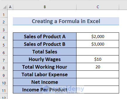
In the following dataset, you can see the values for Sales of Product A, Sales of Product B, Hourly Wages, and Total Working Hour. Now, we have to calculate Total Sales, Total Labor Expense, Net Income, and Income Per Product. To do so, we will create a formula in Excel. Here, we will go through 5 easy methods to do the task, and we have used Excel 365. You can use any available Excel version.
1. Using Constants and Operators to Create a Formula in Excel
In this method, we will use constants and operators to create a formula in Excel. Constants are those values that are used in a calculation. Operators determine the calculation you are performing such as the plus sign for addition (+), minus sign for subtraction (–), asterisk for multiplication (*), and forward slash for division (/).
Steps:
- For our dataset, to find out the Total Sales we need to add Sales of Product A and Sales of Product B.
- In the first place, we will insert an equal sign (=) in cell C6.
- Then, we will type the value of Sales of Product A >> put plus sign (+) >> type the value of Sales of Product B.
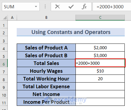
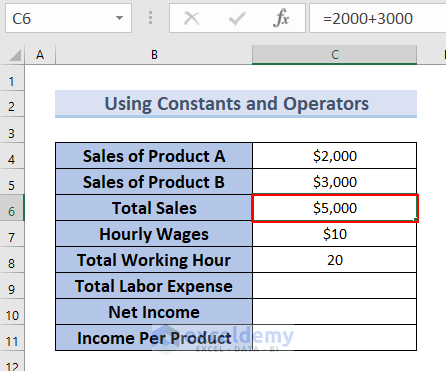
- After that press ENTER.
- Therefore, you can see the result in cell C6.
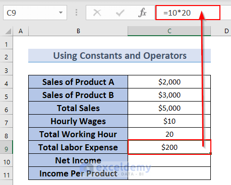
- After that, to find out the Total Labor Expense, we will insert an equal sign (=) in cell C9.
- Then, we will type the value of Hourly Wages >> put an asterisk for multiplication (*) >> type the value of Total Working Hour.
- Afterward, press ENTER.
- As a result, you can see the result in cell C9.
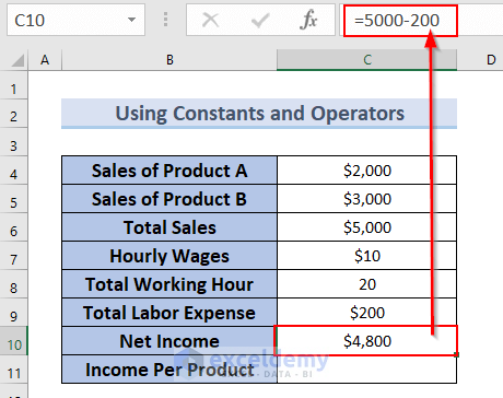
- In addition, to find out the Net Income, we will insert an equal sign (=) in cell C10.
- Furthermore, we will type the value of Total Sales >> put a Subtraction sign (-) >> type the value of Total Labor Expense.
- Afterward, press ENTER.
- As a result, you can see the result in cell C10.
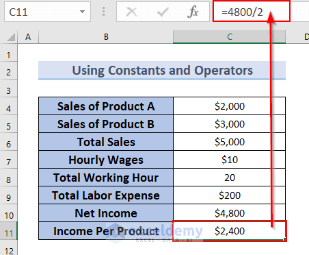
- Furthermore, to find out the Income Per Product, we will insert an equal sign (=) in cell C11.
- Along with that, we will type the value of Net Income >> put the forward slash for division (/) >> type 2.
- Afterward, press ENTER.
- As a result, you can see the result in cell C11.
Read More: How to Create a Formula in Excel without Using a Function
2. Applying Cell References
In this method, we will type cell references to create a formula in Excel. Instead of typing the constant, we can refer to other cells. The benefit of referring cells is that if you make any change in the referred cell, the value used in the calculation will automatically change.
Steps:
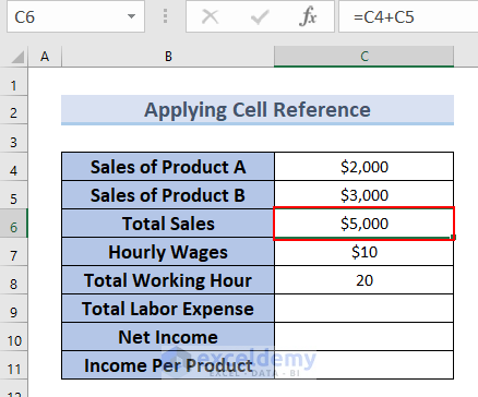
- First of all, to find the Total Sales, put an equal sign (=) in cell C6.
- After that, we will type the reference cell number C4 >> put a plus sign (+) >> type the reference cell number C5.
- The cell you referred to will be highlighted in your worksheet.

- At this point, press ENTER.
- Therefore, you can see the result in cell C6.
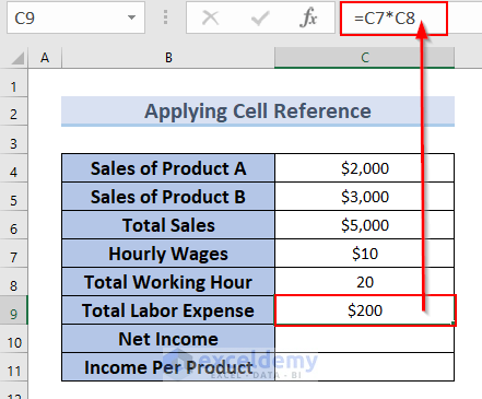
- After that, to find the Total Labor Expense put an equal sign (=) in cell C9.
- After that, we will type the reference cell number C7 >> put an asterisk for multiplication (*) >> type the reference cell number C8.
- The cell you referred to will be highlighted in your worksheet.
- At the moment, press ENTER.
- As a result, you can see the result in cell C6.
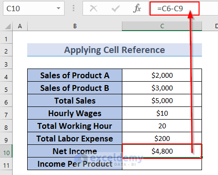
- Then, to find the Net Income put an equal sign (=) in cell C10.
- After that, we will type the reference cell number C6 >> put a subtraction sign (-) >> type the reference cell number C9.
- The cell you referred to will be highlighted in your worksheet.
- Moreover, press ENTER.
- Hence, you can see the result in cell C10.
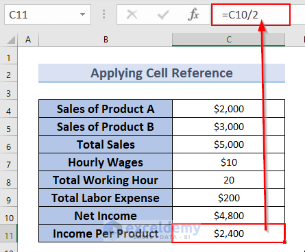
- Finally, to find the Income Per Product put an equal sign (=) in cell C11.
- After that, we will type the reference cell number C10 >> put a forward slash for division (/) >> type 2.
- The cell you referred to will be highlighted in your worksheet.
- Moreover, press ENTER.
- Therefore, you can see the result in cell C11.
Read More: How to Create a Formula in Excel for Multiple Cells
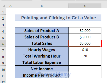
3. Pointing and Clicking to Create a Formula in Excel
In this method, we will use the point-and-click method to create a formula in Excel. Instead of typing the cell number in the formula, you can simply select the cell by pointing and clicking.
Steps:
- First of all, to find the Total Sales, put an equal sign (=) in cell C6.
- After that, we will select the reference cell number C4 by pointing the mouse over cell C4.
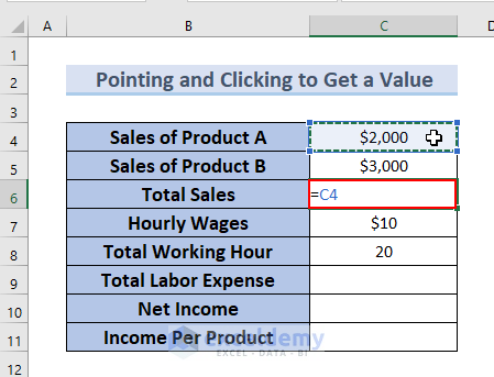
- Then, we put a plus sign (+) >> select the reference cell number C5.
- The cell you referred to will be highlighted in your worksheet.
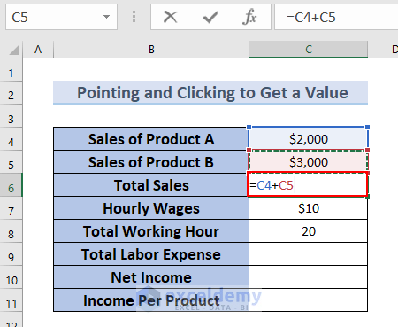
- In addition, press ENTER.
- Therefore, you can see the result in cell C6.
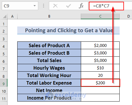
- Moreover, to find the Total Labor Expense put an equal sign (=) in cell C9.
- Afterward, we will select the reference cell number C8 by pointing the mouse over this cell.
- In addition, we will put an asterisk for multiplication (*).
- Then, we will select the reference cell number C7 by pointing the mouse over this cell.
- In addition, press ENTER.
- Therefore, you can see the result in cell C9.
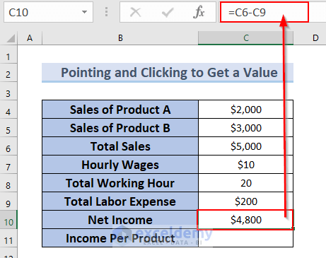
- Moreover, to find the Net Income put an equal sign (=) in cell C10.
- Afterward, we will select the reference cell number C6 by pointing the mouse over this cell.
- In addition, we will put a subtraction sign (-).
- Then, we will select the reference cell number C9 by pointing the mouse over this cell.
- Along with that, press ENTER.
- As a result, you can see the result in cell C10.
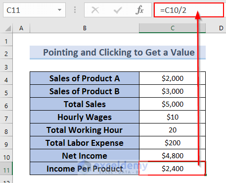
- Finally, to find the Income Per Product put an equal sign (=) in cell C11.
- Afterward, we will select the reference cell number C10 by pointing the mouse over this cell.
- In addition, we will put a forward slash for division (/) >> type 2.
- Along with that, press ENTER.
- Hence, you can see the result in cell C11.
4. Defining Cell’s Name to Create a Formula in Excel
In this method, we will define the cell’s name, and using the names we will create a formula in Excel.
Steps:
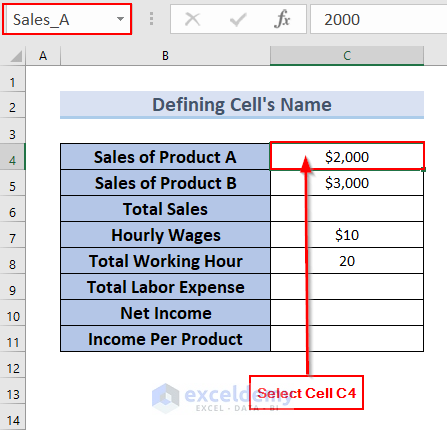
- First, to give a name for cell C4, select cell C4 >> type a name in the Name Box beside the Formula Bar.
- Here, we type Sales_A.
- Then, press ENTER.
- Therefore, cell C4 will have a defined name.
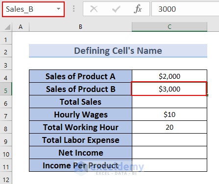
- Furthermore, we will define a name for cell C5 as well.
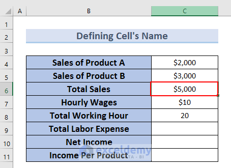
- Later, to find the Total Sales, we will type an equal (=) in cell C6.
- Then, we will type Sales_A >> put a Plus sign (+) >> type Sales_B.

- At this point, press ENTER.
- As a result, you can see the result in cell C6.
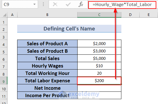
- In a similar way, we define names for cells C8 and C9.
- Here, for C8 we define the name as Hourly_Wage, and for cell C9 we define the name as Total_Labor.
- Next, to find the Total Labor Expense, we will type an equal (=) in cell C9.
- Then, we will type Hourly_Wage >> put an asterisk for multiplication (*) >> type Total_Labor.
- After that, press ENTER.
- As a result, you can see the result in cell C9.
- In addition, we define names for cells C6 and C9.
- Here, for C6 we define the name as Total_Sales, and for cell C9 we define the name as Total_Labor_Expense.
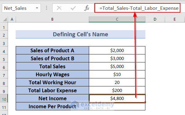
- Next, to find the Net Income, we will type an equal (=) in cell C10.
- Afterward, we will type Total_Sales>> put a subtraction sign (-) >> type Total_Labor_Expense.
- After that, press ENTER.
- Therefore, you can see the result in cell C10.
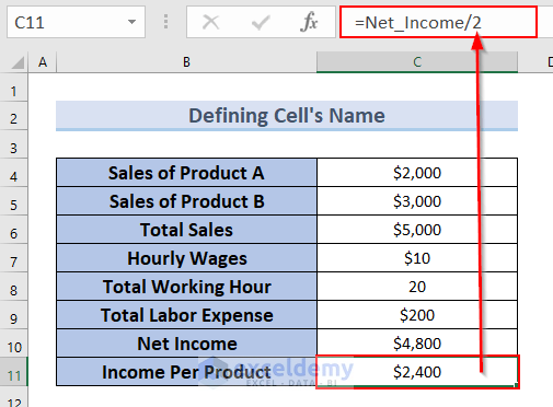
- Moreover, we define the name of cell C10.
- Here, for C10 we define the name as Net_Income.
- Furthermore, to find the Income Per Product we will type an equal (=) in cell C11.
- Afterward, we will type Net_Income >> put a forward slash for division (/) >> type 2.
- After that, press ENTER.
- Hence, you can see the result in cell C11.
5. Creating a Formula by Using Functions
Functions are predetermined formulas that Excel has built. There are thousands of formulas excel has and you can calculate almost any type of calculation by using this formula. Here, we will use the in-built functions of Excel to create a formula.
5.1. Using Insert Function Feature
You can use a formula from the Function wizard to create a formula in Excel.
Steps:
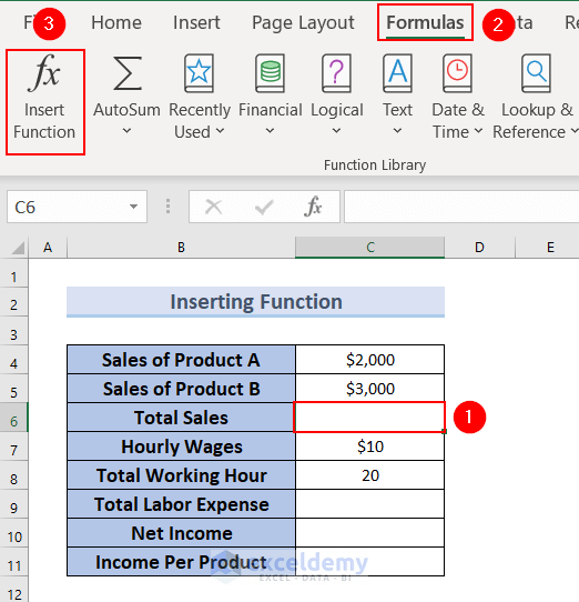
- First of all, we have to select the cell where we want to put the formula.
- Here, we want the SUM function in cell C6 to find the Total Sales.
- Therefore, we click on cell C6.
- Then, we go to the Formulas tab >> select Insert Function.
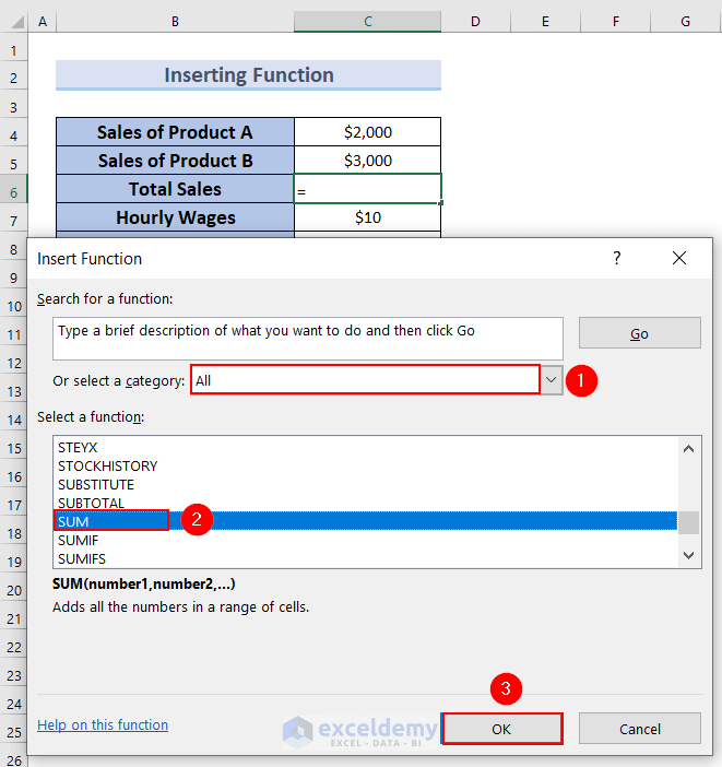
- At this point, an Insert Function dialog box will appear.
- Then, in the Or select a category box, we will select All.
- Here, make sure to select All, this will bring out all the built-in functions of Excel.
- Then, in the Select a Function box >> scroll down until you find the SUM function.
- After that, click on the SUM function >> click OK.
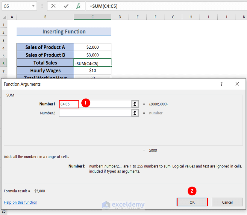
- Then, the Function Arguments dialog box will appear.
- Afterward, in the Number1 box, select the range of cells that you want to sum up.
- Here, we selected cells C4:C5.
- Then, click OK.
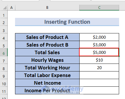
- Therefore, you can see the result in cell C6.
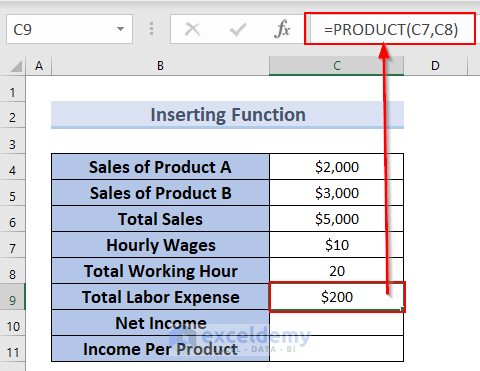
- In a similar way, we use the PRODUCT function for multiplication to find the Total Labor Expense.
- Therefore, you can see the result in cell C9.
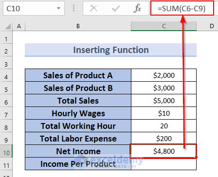
- Since there is no function for subtraction in Excel. You need to use the SUM function to do these calculations.
- Therefore, we use the SUM function for subtraction to find the Net Income.
- Here, we simply put a minus sign (-) before the value of cell C9.
- As a result, you can see the output in cell C10.
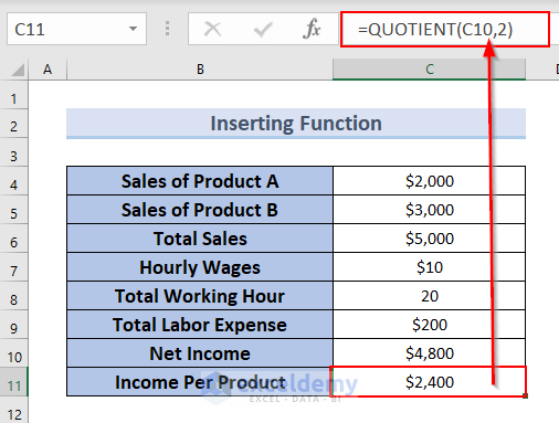
- Along with that, we use the QUOTIENT function for the division to find the Income Per Product.
- Hence, you can see the result in cell C11.
Read More: How to Create a Custom Formula in Excel
5.2. Using Formula Bar
Here, we will use the Formula Bar to insert a function so that we can create a formula in Excel.
Steps:
- In the first place, to find the Total Sales we will use the SUM function.
- Now, to insert the function, we will type an equal sign (=) in cell C6 >> type the SUM function in the Formula Bar and select the cell range (C4:C5).
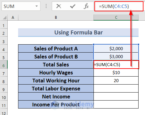
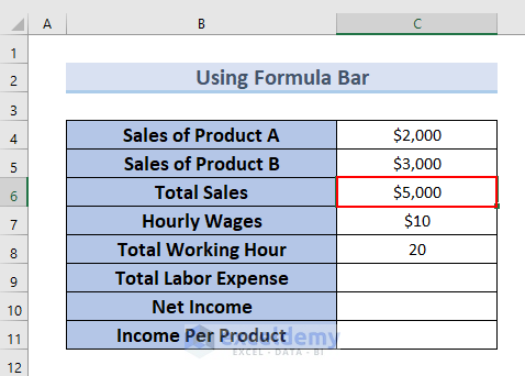
- After that, press ENTER.
- Therefore, you can see the result in cell C6.
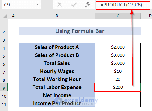
- In a similar way, to find the Total Labor Expense, we type the PRODUCT function in the Formula Bar >> select C7 as the first argument and C8 as the second argument.
- Then, press ENTER.
- Therefore, you can see the result in cell C9.
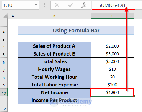
- Moreover, to find the Net Income, we type the SUM function in the Formula Bar >> select cell range.
- Here, since we want subtraction, we put a minus sign (-) before cell C9.
- Then, press ENTER.
- Therefore, you can see the result in cell C10.
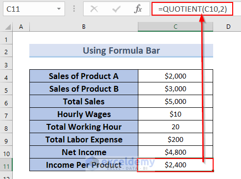
- Finally, to find the Income Per Product, we type the QUOTIENT function in the Formula Bar >> select 10 as the first argument (dividend) and 2 as the second argument (divisor).
- Then, press ENTER.
- Therefore, you can see the result in cell C11.
Read More: How to Apply Formula in Excel for Alternate Rows
How to Create a Formula for Dates in Excel
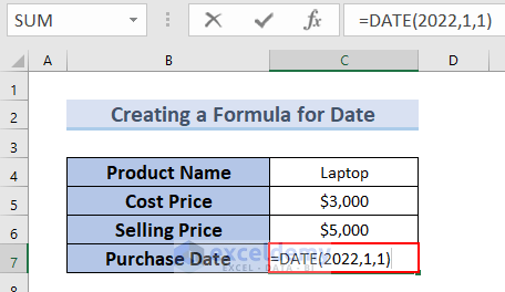
In the following dataset, you can see the Product Name, Cost Price, and Selling Price. Now, we will find the Purchase Date for the product. Here, we will show you how you can create a formula for dates in Excel. We will use the DATE function for this purpose.
Steps:
- First of all, we will type the following formula in cell C7.
=DATE(2022,1,1)- Here, 2022 is the Year, 1 is the Month, and 1 is the Day.
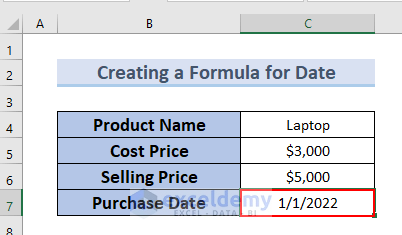
- After that, press ENTER.
- Hence, you can see the result in cell C7.
Practice Section
You can download the above Excel file and practice the explained methods.

You can download the Excel file and practice while reading this article.
Conclusion
Here, we show you 5 easy methods to create a formula in Excel. Thank you for reading this article. We hope it was helpful. If you have any queries, please let us know in the comment section.
How to Create Excel Formulas: Knowledge Hub
- Insert Formula for Entire Column
- Create a Complex Formula
- Create a Conditional Formula
- How to Apply a Formula to Multiple Sheets in Excel
- Use Multiple Excel Formulas in One Cell
- Apply Formula to Entire Column Without Dragging
- Apply Same Formula to Multiple Cells
- Create a Formula Using Defined Names
- Exclude Zero Values with Formula
- Make FOR Loop in Excel Using Formula
- Apply Formula to Entire Column Using Excel VBA
- Use Point and Click Method
<< Go Back to Excel Formulas | Learn Excel
Get FREE Advanced Excel Exercises with Solutions!
