How to Calculate Average Days in Excel (2 Easy Ways)

In Excel, when we need to calculate the average days of different dates depending on our data set, you may find it somewhat difficult. This article will show you how to calculate average days in Excel with two convenient methods.

How to Calculate Average Days in Excel: 2 Easy Approaches

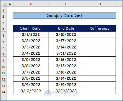
In this article, we will demonstrate to you how to calculate average days in Excel by utilizing the AVERAGE function and the combination of the SUMPRODUCT function and the COUNT function. Let’s suppose we have a sample data set.

1. Utilizing Average Function to Calculate Average Days in Excel

In this section, we will determine the differences between the two dates in the given data set and then we will apply the AVERAGE function to calculate the average days in Excel.

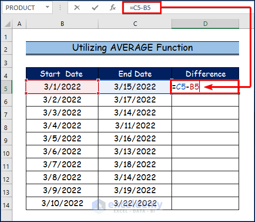
Step 1:

Firstly, select the D5 cell.
Then write down the following formula in the D5 cell.

=C5-B5

After that, press ENTER.

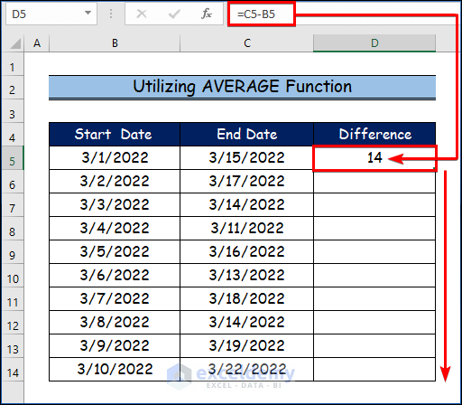
Step 2:

Here, you will see the first difference in the D5 cell between the first end date and the start date.
Then, use the Fill Handle tool and drag it down from the D5 cell to the D14 cell.

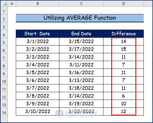
Step 3:

Finally, you will find all the differences between the end date and the start date.

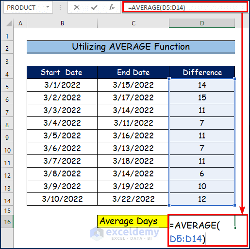
Step 4:

In this part, apply the following average formula in the D16 cell.

=AVERAGE(D5:D14)

After that, hit ENTER.

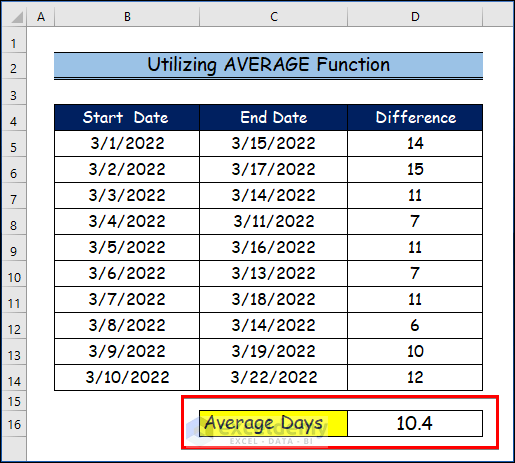
Step 5:

As a result, you will observe the average days in the D16 cell in the below image.

2. Combining SUMPRODUCT and COUNT Functions to Calculate Average Days

In this second section, we will apply the SUMPRODUCT function and the COUNT function at a time to evaluate the average days in Excel. The sum of the products of related ranges or arrays is returned by the SUMPRODUCT function. Although addition, subtraction, and division are also options, multiplication is the default operator. The COUNT function in Excel provides a count of values that are numerical values. Negative numbers, percentages, dates, times, numbers, fractions, and formulas that return numbers are all examples of numbers. Text values and empty cells are discarded.

Step 1:

Firstly, select the D16 cell.
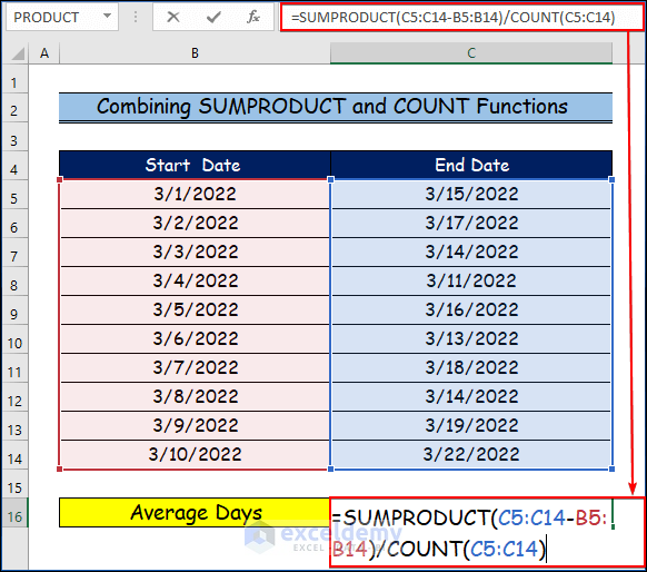
Then, type the following formula here to determine the average days in Excel.

=SUMPRODUCT(C5:C14-B5:B14)/COUNT(C5:C14)

Formula Breakdown

=SUMPRODUCT(C5:C14-B5:B14): This portion of the formula returns the value in terms of the end date and start date by applying the SUMPRODUCT subtraction formula and the value is 104.

=SUMPRODUCT(C5:C14-B5:B14)

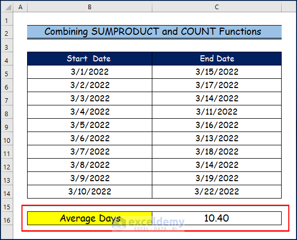
=SUMPRODUCT(C5:C14-B5:B14)/COUNT(C5:C14): This is a combination of the SUMPRODUCT function and the COUNT function which returns the final result of average days 10.4.

=SUMPRODUCT(C5:C14-B5:B14)/COUNT(C5:C14)

After that, press ENTER.

Step 2:

Consequently, you will see the following result of the average days in Excel.

Download Practice Workbook

You may download the following Excel workbook for better understanding and practice it by yourself.

Calculate Average Days.xlsx

Conclusion

In this article, we’ve covered 2 handy methods to calculate average days in Excel. We sincerely hope you enjoyed and learned a lot from this article. Additionally, If you have any questions, comments, or recommendations, kindly leave them in the comment section below.