While dealing with the sales of a company, sometimes we need to forecast the sales of that company to predict the profit or loss. In this case, Microsoft Excel can be a handy tool for you. Today I am going to show you five easy and suitable steps to calculate forecast confidence interval in Excel effectively with appropriate illustrations.
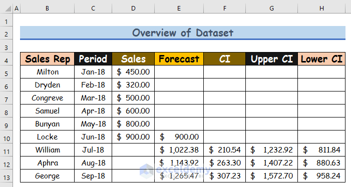
Let’s say, we have a dataset that contains information about the sales forecast of the XYZ group. From our dataset, we will calculate forecast confidence intervals in Excel. We can easily calculate forecast confidence intervals in Excel by using FORECAST.ETS, FORECAST.ETS.CONFINT functions and mathematical formulas. Here’s an overview of the dataset for today’s task.
Step 1: Creating Dataset Header to Calculate Forecast Confidence Interval in Excel
In the first step, you will have to insert headers to calculate the forecast confidence interval and then format them in Excel. The header columns are the Sales representative’s name, Period, Sales in several periods, Forecast, Confidence Intervals (CI), Upper Confidence Intervals, and Lower Confidence Intervals. So, our dataset becomes as below.

Step 2: Applying FORECAST.ETS Function to Calculate Forecast Confidence Interval in Excel
In this step, we will apply the FORECAST.ETS function to calculate the forecast. From our dataset, we can easily do that. Firstly, we will calculate the forecast for July. Hence, we will calculate the forecast for the rest of the months in column E. Let’s follow the instructions below to learn!
- First of all, select cell E11 and write down the below FORECAST.ETS function in that cell.
=FORECAST.ETS(C11,$D$5:$D$10,$C$5:$C$10,1,1,1)- Where C11 is the target_date, $D$5:$D$10 is the values, $C$5:$C$10 is the timeline, first 1 is the seasonality, second 1 is the data_completion, and the rest 1 is the aggregation of the FORECAST.ETS function.
- We use the Dollar sign ($) for absolute reference.
- Hence, simply press Enter on your keyboard. As a result, you will get the estimated forecast of July 2018 which is the return of the FORECAST.ETS function. The return is $1,022.38.

- Hence, AutoFill the FORECAST.ETS function to the rest of the cells in column E.

Note: Accuracy of Excel FORECAST Function
The survey results are always within ± 5%, ± 15%, or any other percent; they are never a precise figure. You can’t rely on a forecast if you don’t know how accurate it is. The world is full of uncertainty. In Excel, there isn’t a straightforward way to assess sales forecasting accuracy, or at least not one that wouldn’t require years to develop.
Step 3: Using FORECAST.ETS.CONFINT Function
Now, we will calculate the Confidence Intervals using the FORECAST.ETS.CONFINT function in Excel. From our dataset, we can easily calculate the Confidence Intervals. Let’s follow the instructions below to learn!
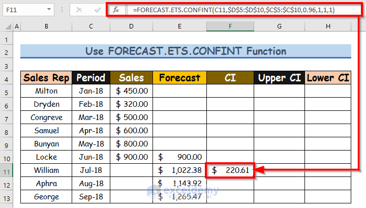
- First of all, select cell F11 and write down the below FORECAST.ETS.CONFINT function in that cell.
=FORECAST.ETS.CONFINT(C11,$D$5:$D$10,$C$5:$C$10,0.95,1,1,1)- Where C11 is the target_date, $D$5:$D$10 is the values, $C$5:$C$10 is the timeline, 96 is the Confidence_level, first 1 is the seasonality, second 1 is the data_completion, and the rest 1 is the aggregation of the FORECAST.ETS.CONFINT function.
- We use the Dollar sign ($) for absolute reference.
- Hence, simply press Enter on your keyboard. As a result, you will get the estimated forecast which is the return of the FORECAST.ETS.CONFINT function. The return is $220.61.
- Hence, AutoFill the FORECAST.ETS.CONFINT function to the rest of the cells in column F.

Step 4: Calculating Upper Confidence Interval
Here, we will learn how to calculate the Upper Confidence Intervals. Let’s follow the instructions below to learn!
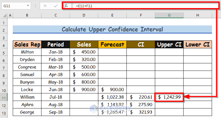
- First of all, select cell G11 and write down the below mathematical formula in that cell.
=E11 + F11- Where E11 is the forecast, F11 is the Confidence Intervals.
- Hence, simply press Enter on your keyboard. As a result, you will get the Upper Confidence Intervals which is the return of the mathematical formula. The return is $1,242.99.
- Hence, AutoFill the formula to the rest of the cells in column G.

Step 5: Calculating Lower Confidence Interval
Last but not least, we will calculate the Lower Confidence Interval. Let’s follow the instructions below to learn!
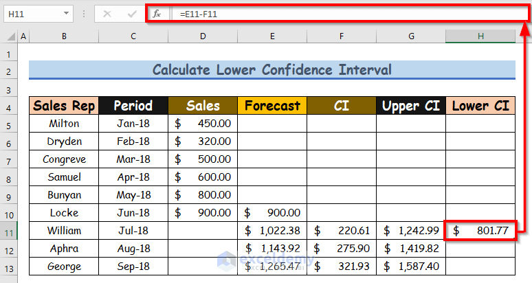
- First of all, select cell H11 and write down the below mathematical formula in that cell.
=E11 - F11- Where E11 is the forecast, F11 is the Confidence Intervals.
- Hence, simply press Enter on your keyboard. As a result, you will get Lower Confidence Intervals which is the return of the mathematical formula. The return is $801.77.
- Hence, AutoFill the formula to the rest of the cells in column H.

Bottom Line
👉 #N/A! the error arises when the formula or a function in the formula fails to find the referenced data.
👉 #DIV/0! the error happens when a value is divided by zero(0) or the cell reference is blank.
Download Practice Workbook
Download this practice workbook to exercise while you are reading this article.
Conclusion
I hope all of the suitable methods mentioned above to calculate forecast confidence interval will now provoke you to apply them in your Excel spreadsheets with more productivity. You are most welcome to feel free to comment if you have any questions or queries.
Related Articles
- How to Make a Confidence Interval Graph in Excel
- How to Calculate 99 Confidence Interval in Excel
- How to Find Confidence Interval in Excel for Two Samples
- Linear Regression Confidence Interval in Excel
- How to Calculate Confidence Interval for Slope in Excel
- How to Find Upper and Lower Limits of Confidence Interval in Excel
- How to Calculate 95 Percent Confidence Interval in Excel
- How to Calculate 90 Percent Confidence Interval in Excel
<< Go Back to Confidence Interval Excel | Excel for Statistics | Learn Excel
Get FREE Advanced Excel Exercises with Solutions!
