⏷1. Using Conditional Formatting to Find & Highlight Duplicates in Excel
⏵1.1. Highlighting Duplicates in Excel with Duplicate Values Command
⏵1.2. Getting Duplicate Values with COUNTIF Function
⏵1.3. Finding & Highlighting Triplicate Cells (3 Occurrences)
⏵1.4. Highlighting Duplicate Values from Two Different Worksheets
⏵1.5. Applying COUNTIFS Function to Find & Highlight Duplicate Rows
⏷2. Using Excel Formula to Find Duplicate Values and Return Conditional Outputs
⏵2.1. Applying COUNTIF Function to Find Duplicate Values and Return TRUE or FALSE
⏵2.2. Combining IF and COUNTIF Functions and Return the Text ‘Duplicate’
⏷3. Returning the Number of Occurrences & Finding Duplicates in Excel
⏵3.1. Finding Number of Duplicate Instances with COUNTIF Function
⏵3.2. Using SUM Function to Count Duplicate Occurrences
⏵3.3. Joining IF and SUM Functions to Count Duplicates
⏵3.4. Counting Number of Duplicate Rows with COUNTIFS Function
⏵3.5. Using SUMPRODUCT Function to Find Number of Duplicate Rows
⏷4. Using Excel Functions to Find Duplicate Rows From Two or Multiple Columns
⏵4.1. Combining IF and COUNTIFS Function to Find Duplicate Rows
⏵4.2. Joining IF & SUMPRODUCT Functions to Find Duplicate Rows
⏷5. Finding Duplicates in a Column Excluding 1st Occurrence
⏷6. Finding Case-Sensitive Duplicates with Excel Formula
⏷7. Finding Duplicates from Two or Three Columns in Excel
⏵7.1. Finding Duplicates From Two Columns
⏵7.2. Finding Duplicates From Three or More Columns
⏷8. Finding Duplicate Values Across Two Sheets in Excel
⏷9. Finding Duplicates Between Two Excel Workbooks
⏷10. Applying VBA Macro to Find Duplicates in Excel
⏷11. Applying Excel Formula to Find & Return Duplicate Values
⏵11.1. Combining IF and COUNTIF Functions to Get Duplicate Values
⏵11.2. Return Duplicate Values Only Once
⏵11.3. Joining IFERROR and VLOOKUP Functions to Return Duplicates from Two Sheets
⏷How to Select, Copy, Move, Remove or Hide Duplicates in Excel after Finding Them?
⏷Tips to Find Duplicates in Excel
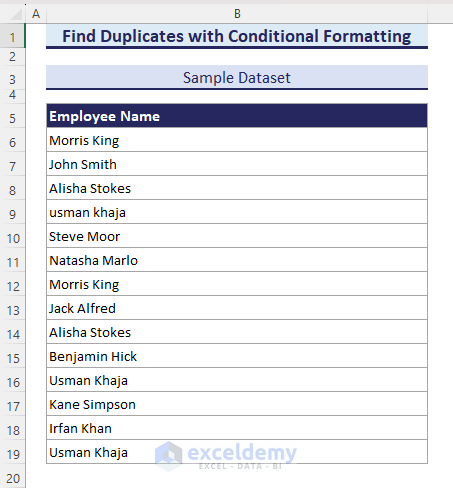
Method 1 – Using Conditional Formatting to Find & Highlight Duplicates in Excel
Considering the below dataset, we will show 5 applications of the Conditional Formatting tool to find duplicate values.
- Use of Duplicate Values command
- Application of the COUNTIF function
- Finding triplicates
- Marking duplicates compared with another worksheet
- Use of COUNTIFS to get duplicate rows
1.1. Duplicate Values Command
Microsoft Excel’s Conditional Formatting offers an easy way to find and highlight duplicates.
Follow these steps:
- Select the data range B6:B19.
- Go to the Home tab, select Conditional Formatting, click on Highlight Cells Rules and choose Duplicate Values.
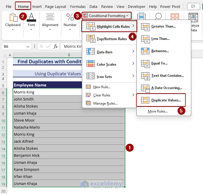
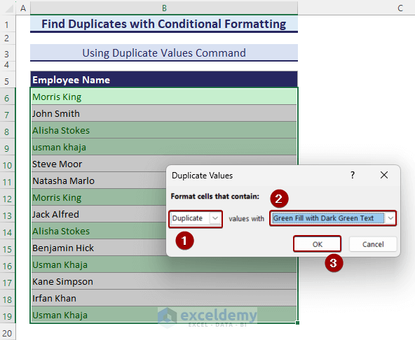
- The Duplicate Values dialog box will show up.
- Select Duplicate and in the values with field, choose Green Fill with Dark Green.
- Click OK.
- All the duplicate cells will be highlighted.
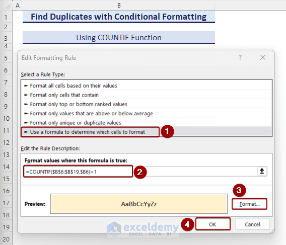
1.2. Application of COUNTIF Function
Use the COUNTIF formula with Conditional Formatting to highlight duplicate values.
Here’s how:
- Select data range B6:B19.
- Got to the Home tab, select Conditional Formatting and click on New Rule.
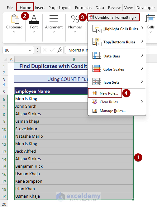
- Insert the following formula in the Format values where this formula is true field.
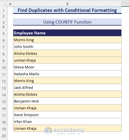
=COUNTIF($B$6:$B$19,$B6)>1- Select fill color from the Format button and click OK.
- Duplicate values will be highlighted.
1.3. Finding & Highlighting Triplicate Cells (3 Occurrences)
- Triplicate refers to three instances of a particular value in a dataset.
- To find triplicates, use the Conditional Formatting tool with the COUNTIF function.
- Apply the following COUNTIF formula in the Edit Formatting Rule dialog box:
=COUNTIF($B$6:$B$19,$B6)=3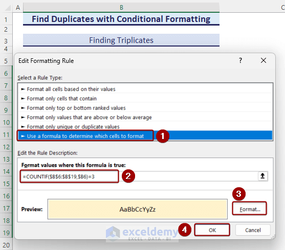
- As a result, Usman Khaja (appearing three times in the Employee Name list) gets highlighted.
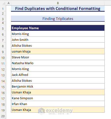
- Note that Morris King appears twice but isn’t highlighted because the formula was customized to find a minimum of three instances of the same value.
1.4. Highlighting Duplicate Values from Two Different Worksheets
- We have two separate worksheets containing employee names.
- Compare current employee names with Dataset 2 (shown on the left) and highlight duplicate names on the right portion of the image.
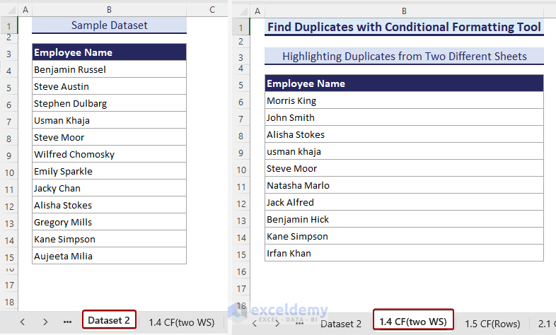
- Apply the COUNTIF formula in the Edit Formatting Rule dialog box:
=COUNTIF('Dataset 2'!$B$4:$B$15,$B6)>0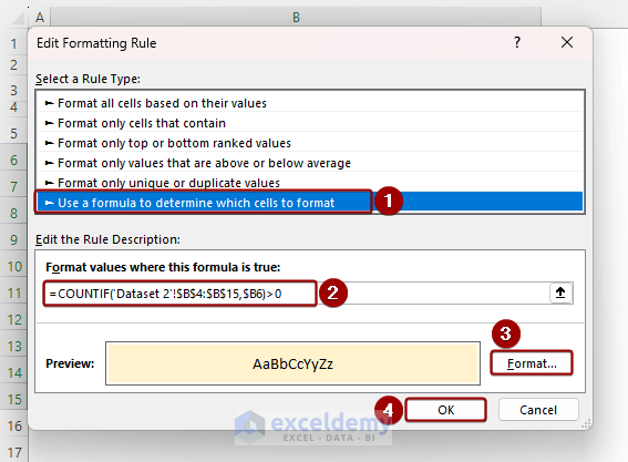
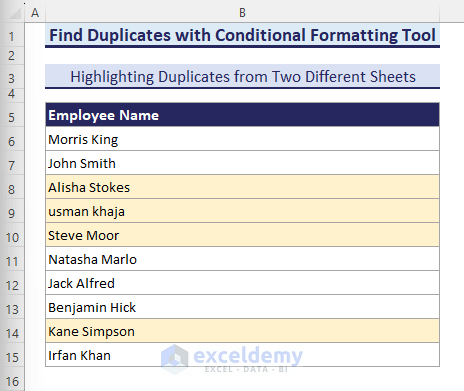
- All matched names will be highlighted.
1.5. Applying COUNTIFS Function to Find & Highlight Duplicate Rows
- Use the COUNTIFS function to find and highlight duplicate rows in Excel.
- COUNTIFS allows multiple criteria for matching.
- Apply the COUNTIFS function as follows:
=COUNTIFS($B$6:$B$19,$B6,$C$6:$C$19,$C6,$D$6:$D$19,$D6,$E$6:$E$19,$E6)>1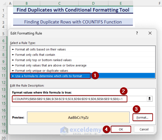
- This identifies all duplicate rows.
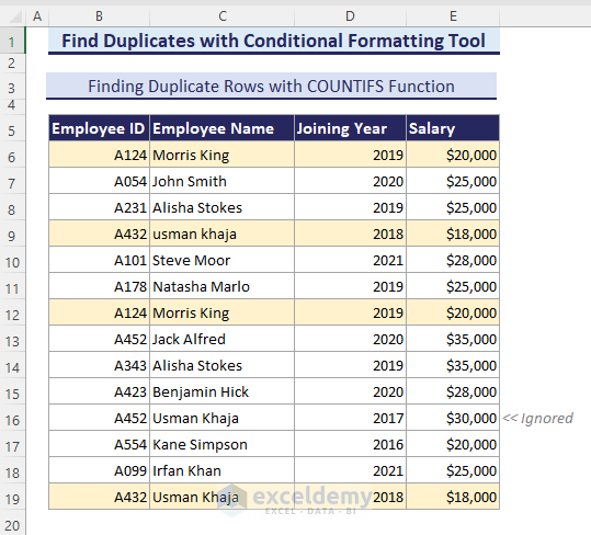
- Note that Usman Khaja also appears in cell C16 but isn’t highlighted due to mismatched Employee ID, Joining Year, and Salary.
Method 2. Using Excel Formula to Identify Duplicate Values and Return Conditional Outputs
In this section, we will discuss the use of Excel functions to find duplicates in Excel and return conditional texts like TRUE, FALSE, Duplicate, or keep the output cell blank. To figure out duplicate values we will use:
- The COUNTIF function, and
- A combination of IF and COUNTIF functions.
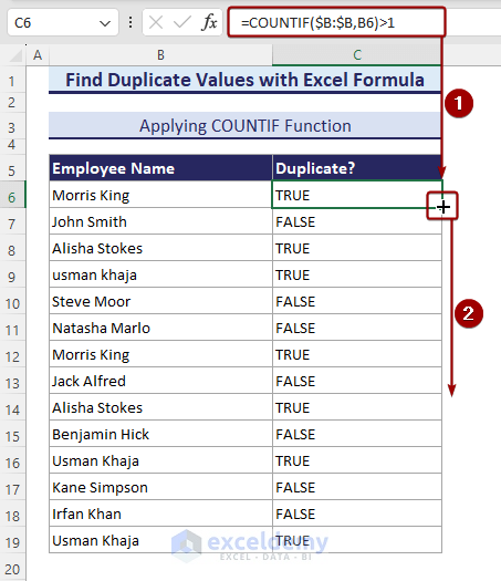
2.1. Using COUNTIF Function to Determine Duplicate Values and Return TRUE or FALSE
- The COUNTIF function calculates the number of occurrences within a specified range.
- By applying the following formula in cell C6, we obtain TRUE for duplicate values:
=COUNTIF($B:$B,B6)>1- Drag down the Fill Handle tool to copy the formula into adjacent cells.
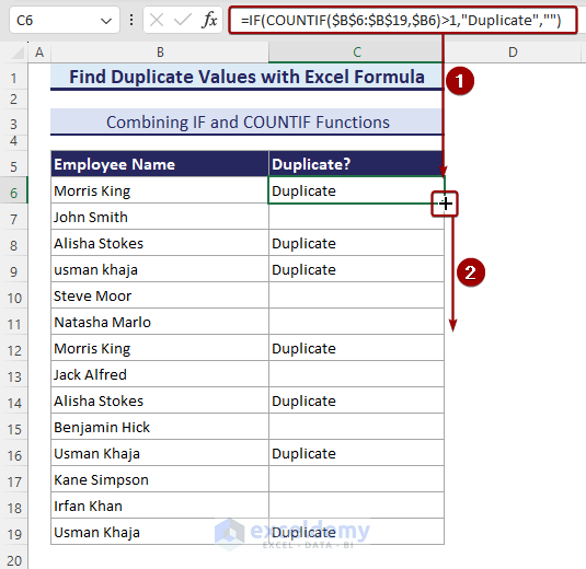
2.2. Combining IF and COUNTIF Functions to Display ‘Duplicate’
- The IF function is a logical function that writes Duplicate when it encounters TRUE (which comes from the COUNTIF function).
- Enter the following formula in cell C6 to achieve this:
=IF(COUNTIF($B$6:$B$19,$B6)>1,"Duplicate","")- Use the Fill Handle tool to extend this across other cells.
Method 3 – Returning the Number of Occurrences & Finding Duplicates in Excel
In this segment, we will discuss how to return the number of occurrences and find duplicates in Excel. There are 5 useful approaches to count the number of occurrences while finding duplicates.
- Enter of the COUNTIF function
- Application of the SUM function
- Combination of IF and SUM functions
- Counting instances of rows with the COUNTIFS function
- Use of SUMPRODUCT functions for counting row instances.
3.1. Using the COUNTIF Function
- The COUNTIF function allows you to count occurrences within a specified range.
- To find duplicate instances, insert the following formula in cell C6:
=COUNTIF($B$6:$B$19,$B6)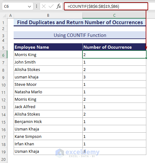
3.2. Using SUM Function to Count Duplicate Occurrences
- The SUM function provides an alternative method for counting duplicate values.
- Enter the following formula in cell C6 to obtain the outcome:
=SUM(--($B$6:$B$19 = $B6))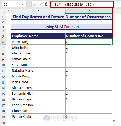
3.3. Combining IF and SUM Functions to Count Duplicates
- By combining the IF and SUM functions, you can efficiently find duplicate instances.
- Apply the following formula in cell C6:
=SUM(IF($B$6:$B$19=$B6,1,0))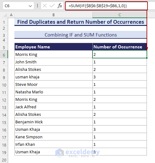
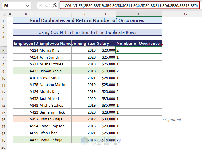
3.4. Counting Duplicate Rows with the COUNTIFS Function
- The COUNTIFS function considers multiple criteria to count instances of duplicate rows.
- Enter the formula below to obtain duplicate rows’ instances:
=COUNTIFS($B$6:$B$19,$B6,$C$6:$C$19,$C6,$D$6:$D$19,$D6,$E$6:$E$19,$E6)- Note that the entry for Usman Khaja in cell C16 is ignored due to differences in employee ID, joining year, and salary.
3.5. Using the SUMPRODUCT Function for Duplicate Rows
- The SUMPRODUCT function provides an alternative approach to finding occurrences of duplicate rows.
- Enter the following formula in cell C6:
=SUMPRODUCT(($B$6:$B$19=$B6)*1,($C$6:$C$19=$C6)*1,($D$6:$D$19=$D6)*1)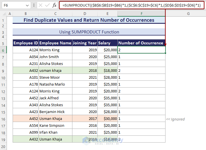
Method 4 – Finding Duplicate Rows in Excel Across Multiple Columns
In this section, we will show you how to find duplicate rows from two or multiple columns in Excel. To do so we will use:
- Combination of IF and COUNTIFS functions
- Application of SUMPRODUCT function
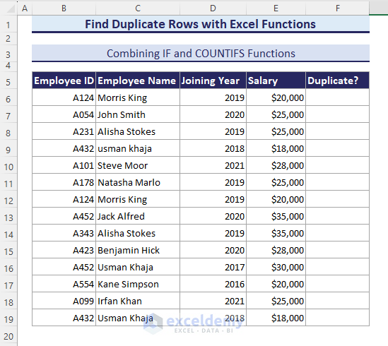
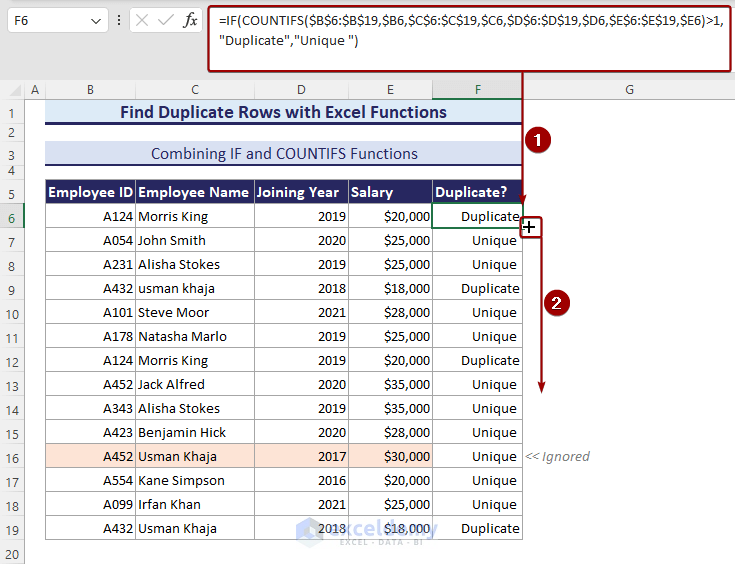
4.1. Combining IF and COUNTIFS Function to Find Duplicate Rows
- The combination of COUNTIFS and IF functions helps find duplicate rows.
- The COUNTIFS function counts instances of rows based on multiple criteria.
- Enter the following formula in cell F6 to label duplicates as Duplicate or Unique:
=IF(COUNTIFS($B$6:$B$19,$B6,$C$6:$C$19,$C6,$D$6:$D$19,$D6,$E$6:$E$19,$E6)>1,"Duplicate","Unique ")- Use the Fill Handle tool to copy the formula in the adjacent cells.
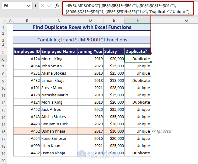
4.2. Joining IF & SUMPRODUCT Functions
- Similar to the previous method, we can use IF and SUMPRODUCT functions together.
- The SUMPRODUCT function calculates the sum of products of corresponding ranges or arrays.
- Enter the following formula in cell F6:
=IF(SUMPRODUCT(($B$6:$B$19=$B6)*1,($C$6:$C$19=$C6)*1,($D$6:$D$19=$D6)*1,($E$6:$E$19=$E6)*1)>1,"Duplicate","Unique")- Autofill the rest of column F using the Fill Handle tool.
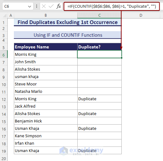
Method 5 – Excluding 1st Occurrence in a Column
- The IF-COUNTIF formula not only finds duplicates including the first instance but also excludes it.
- Enter the following formula in cell C6:
=IF(COUNTIF($B$6:$B6, $B6)>1, "Duplicate", "")- Autofil using the Fill Handle tool.
-
- This formula considers the first occurrence as unique.
- For example, in B9, B16, and B19, Usman Khaja appears three times, but the formula labels only the second and third instances as Duplicate.
- Look carefully, there are 3 instances of Usman Khaja in B9, B16 & B19 The formula will return Duplicate only for the 2nd and 3rd instances and the 1st one will be excluded.
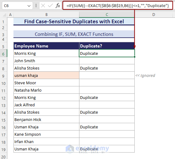
Method 6 – Finding Case-Sensitive Duplicates
- To account for case sensitivity, we’ll use the EXACT function.
- If there’s more than one instance of a case-sensitive value, the formula will return Duplicate.
- Enter the following formula in cell C6:
=IF(SUM((--EXACT($B$6:$B$19,B6)))<=1,"","Duplicate")- Fill the rest of the adjacent cells using the Fill Handle tool.
This ensures that usman khaja in B9 is ignored due to case sensitivity.
Method 7 – Finding Duplicates from Two or Three Columns in Excel
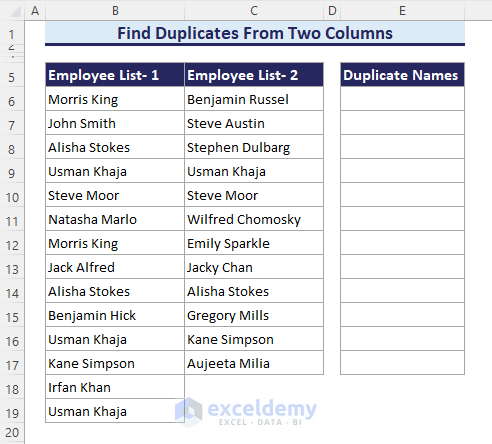
7.1. Finding Duplicates From Two Columns
To find duplicates from the two columns, we will show you two approaches. They are:
- Use of VLOOKUP function
- Combination of UNIQUE, FILTER, and COUNTIF functions
i. Using VLOOKUP Function
- Apply the Excel VLOOKUP function to find duplicate values.
- Look up values from Employee List-2 in Employee List-1.
- If a value is not found, replace it with a dash (“-”) using the IFERROR function.
- Enter the following formula in cell E6 and drag it down using the Fill Handle tool:
=IFERROR(VLOOKUP(C6,$B$6:$B$19,1,FALSE),"-")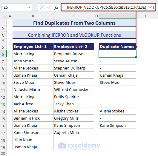
ii. Combining UNIQUE, FILTER and COUNTIF Functions
- Use the FILTER function (available in Excel 2021 and Microsoft 365) to find duplicates.
- Obtain the outcome in an array format by combining FILTER and UNIQUE functions.
- Enter the following formula in cell E6:
=UNIQUE(FILTER(B6:B19,COUNTIF(C6:C17,B6:B19)>0))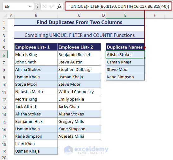
7.2. Finding Duplicates From Three or More Columns
- Use the combination of FILTER and COUNTIF functions.
- Filter duplicates from Employee List-1 and Employee List-2.
- Match the obtained duplicates with Employee List-3.
- Enter the following formula in cell F6 to return the output in an array format:
=FILTER(FILTER(B6:B19,COUNTIF(C6:C17,B6:B19)>0),COUNTIF(D6:D14,FILTER(B6:B19,COUNTIF(C6:C17,B6:B19)>0))>0)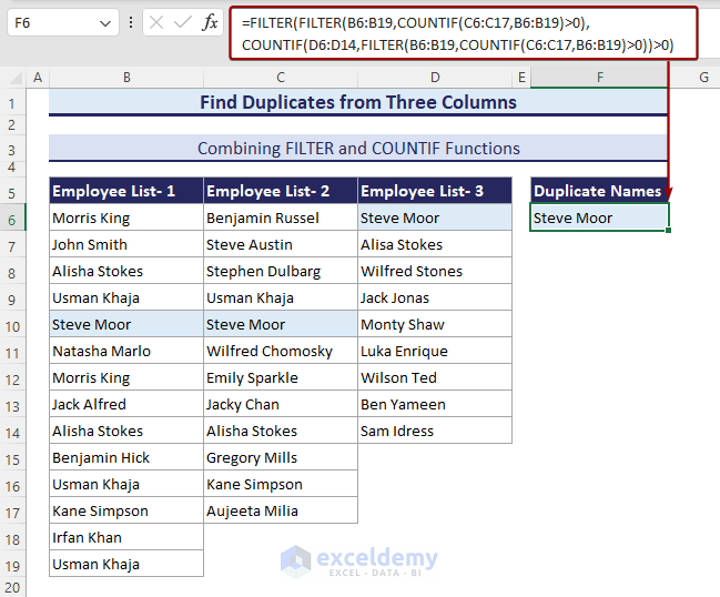
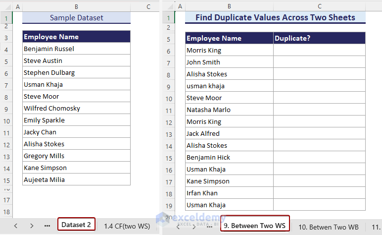
8. Finding Duplicate Values Across Two Sheets in Excel
- Compare two separate worksheets (Dataset 1 and Dataset 2).
- Match Employee names and return duplicate names.
- Use the combination of ISNUMBER and MATCH functions.
- Enter the following formula in cell C6 to return a TRUE-FALSE statement:
=ISNUMBER(MATCH($B6,'Dataset 2'!B4:B15,0))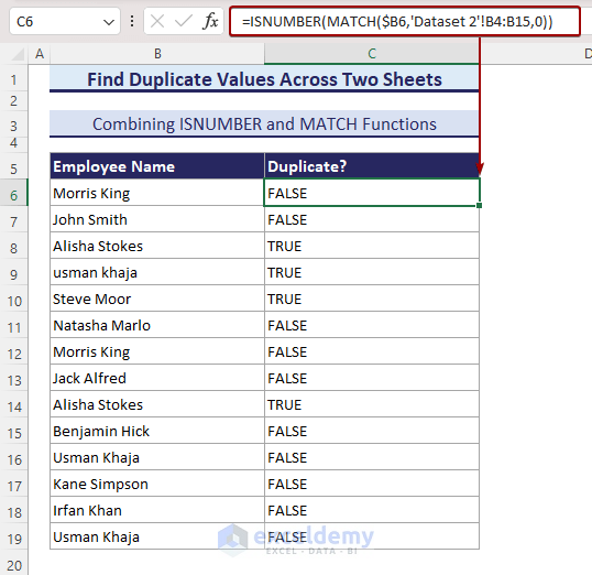
Method 9 – Finding Duplicates Between Two Excel Workbooks
- Compare two separate workbooks (‘Find Duplicates’ and ‘Source Data’).
- Match current Employee names with the new workbook (‘Source Data’) to find duplicate names.
- Combine IF and COUNTIF functions.
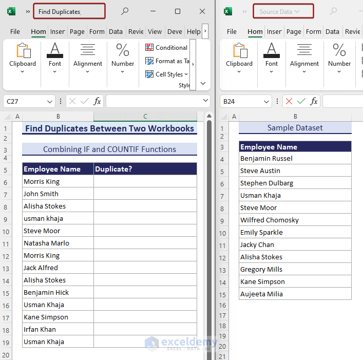
- Enter the following formula in cell C6 to return a TRUE-FALSE statement:
=IF(COUNTIF('[Source Data.xlsx]Dataset3'!$B$4:$B$15,$B6),TRUE,FALSE)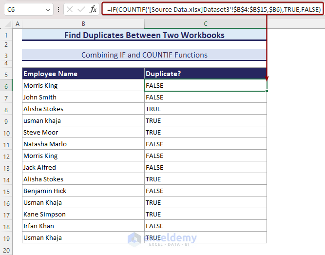
Note:
- Open both workbooks simultaneously to avoid a #VALUE error.
- Ensure the correct file directory when applying the formula.
Method 10 – Using VBA Macro to Find Duplicates in Excel
In this section, we’ll demonstrate how to find duplicates from a column using VBA Macro in Excel. Excel’s VBA Macro tool is essential for identifying duplicates in extensive datasets, multiple worksheets, and multiple workbooks automatically. Although the process is somewhat complex, we’ll guide you through applying VBA Macro to find duplicates in Excel.
- Enter the following VBA code in a Module and Save it:
Sub find_duplicates()
'Developed by MD_Tanvir_Rahman, ExcelDemy
Dim rng As Range
Dim Output_rng As Range
Dim i As Integer
Dim j As Integer
Dim outputRow1 As Integer
Dim foundMatch As Boolean
Dim alreadyFound As Boolean

Set rng = Application.InputBox("Select Your Input Range:", Type:=8)
Set Output_rng = Application.InputBox("Select Your Output Range:", Type:=8)
outputRow1 = 1

For i = 1 To rng.Rows.Count
    foundMatch = False
    alreadyFound = False
    For j = 1 To outputRow1 - 1
        If Output_rng.Cells(j, 1).Value = rng.Cells(i, 1).Value Then
            alreadyFound = True
            Exit For
        End If
    Next j
    If Not alreadyFound Then
        For j = i + 1 To rng.Rows.Count
            If rng.Cells(i, 1).Value = rng.Cells(j, 1).Value Then
                foundMatch = True
                Exit For
            End If
        Next j
        If foundMatch Then
            Output_rng.Cells(outputRow1, 1).Value = rng.Cells(i, 1).Value
            outputRow1 = outputRow1 + 1
        End If
    End If
Next i

End Sub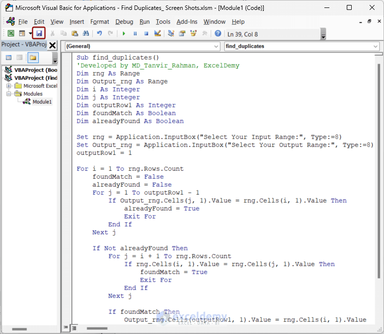
- Go to the Developer tab, select Macros, choose find_duplicates and click on Run.
- Select the input range and output range.
- You will obtain the duplicate names.
Method 11 – Using Excel Formula to Find & Return Duplicate Values
Now we will explain how to find and return duplicate values using Excel formulas. To do so, we’ll show 3 approaches, they are:
- Combination of IF and COUNTIF functions
- Use of SORT and FILTER functions
- Application of VLOOKUP and COUNTIF functions
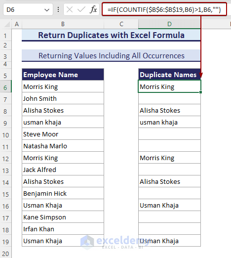
11.1. Combining IF and COUNTIF Functions
- This non-array formula identifies duplicate values.
- Enter the following IF-COUNTIF formula in cell D6 to return duplicate names if found:
=IF(COUNTIF($B$6:$B$19,B6)>1,B6,"")- Autofill the rest of the cells in Column D to get other outputs.
11.2. Combining UNIQUE, FILTER and COUNTIF Functions
- This array formula returns duplicate values only once.
- Enter the following formula in cell D6:
=UNIQUE(FILTER(B6:B19,COUNTIF(B6:B19,B6:B19)>1))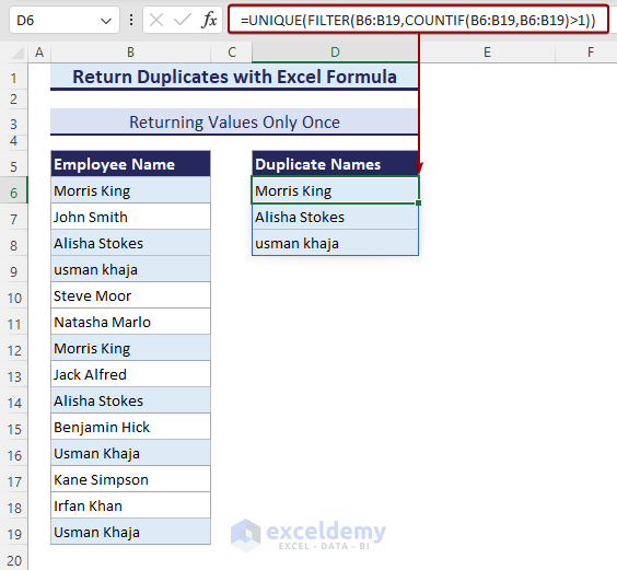
11.3. Using IFERROR and VLOOKUP Functions to Return Duplicates from Two Sheets
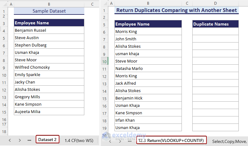
- Suppose we have two separate worksheets. We’ll compare Employee names in the worksheet named Dataset 2 and return duplicate names.
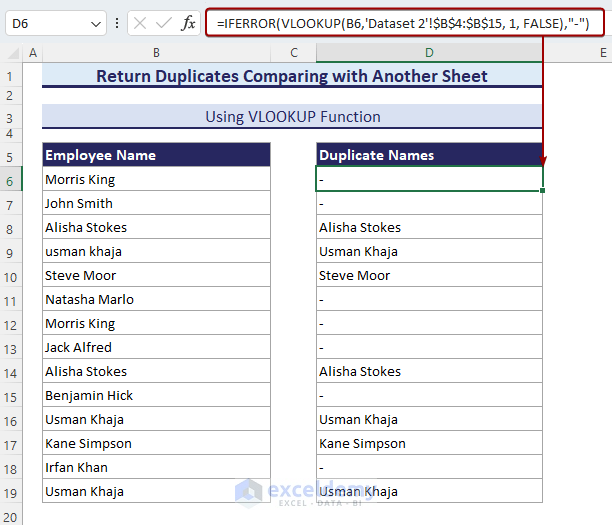
- Enter the following VLOOKUP formula in cell D6 and drag it down:
=IFERROR(VLOOKUP(B6,'Dataset 2'!$B$4:$B$15, 1, FALSE),"-")Note:
- When VLOOKUP is unable to find values, it returns a #N/A error. So, we apply the IFERROR function to omit the error.
- The VLOOKUP function returns only 1st and single value from a column.
- When you apply VLOOKUP in a dataset containing multiple columns, it searches for values in the leftmost column of a range/table and returns the value of the same row of another column to the right.
How to Select, Copy, Move, Remove or Hide Duplicates in Excel after Finding Them
Throughout the article we’ve learned to find duplicates, the number of instances, and return them. Now we will show the process of selecting, copying, moving, removing, and hiding duplicate data after finding them in Excel.
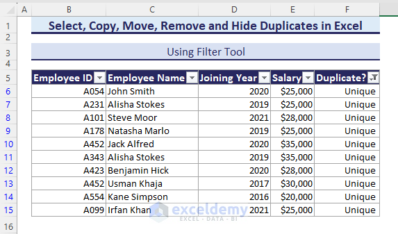
Filter Duplicates
- Select the range containing your data (e.g., B5:F5).
- Go to the Home tab, click Editing, and choose Sort & Filter > Filter.
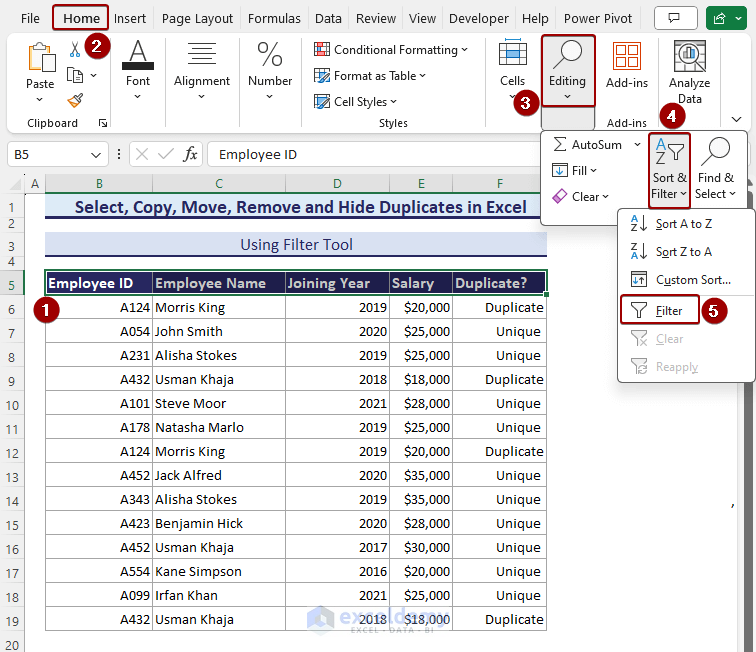
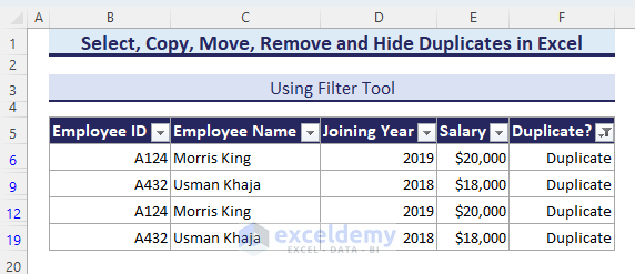
- In the filter drop-down for each column, select Duplicate and click OK. This will display all duplicate rows.
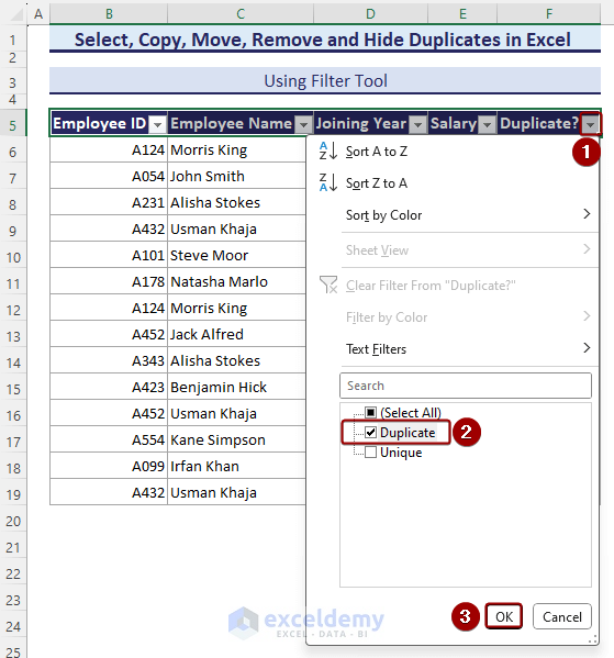
Therefore, all the duplicate rows will show up.
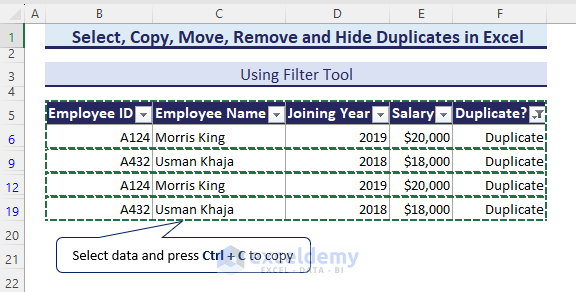
Copy Duplicates
- Press the Ctrl + C keys to copy the duplicate data.
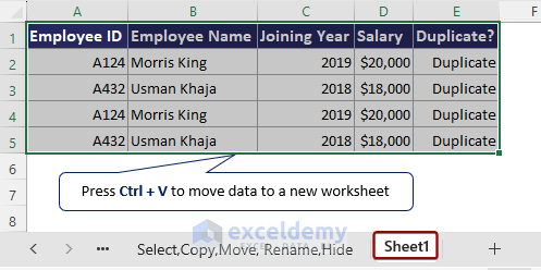
Move Duplicates
- Create a new worksheet.
- Press Ctrl + V to move the duplicate data to the new sheet.
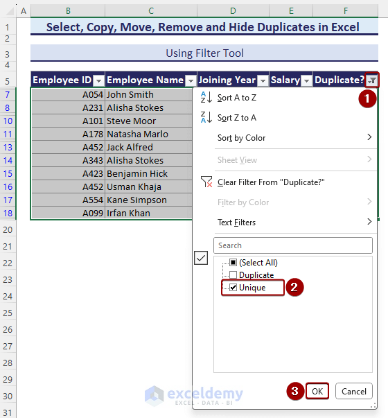
Hide Duplicates
- In the filter drop-down, choose Check Unique only and click OK.
Delete Duplicates
- Select the duplicate data.
- Right-click and choose Delete Row.
- Confirm in the Microsoft Excel dialog box.
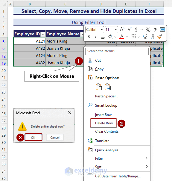
- As a result, we will obtain all the values excluding duplicates.
Tips to Find Duplicates in Excel
Here are some tips for finding duplicates in Excel:
- Consistent Formatting: Ensure consistent formatting and data types to match entries with minor differences.
- Same Order Arrangement: Arrange data in the same order across worksheets for easier duplicate identification.
- Remove Unnecessary Blanks: Eliminate unnecessary rows, columns, and cells to maintain accuracy.
- Use Formulas: Excel formulas can help, even if they seem challenging initially.
- Routine Checks: Regularly check for duplicates, especially in large datasets.
- Learn More About Excel: Explore tutorials and practice different functions to enhance your Excel skills.
Download Practice Workbook
You can download the practice workbook from here:
Find Duplicates in Excel: Knowledge Hub
- Formula to Find Duplicates in Excel
- How to Find Duplicate Values Using VLOOKUP in Excel
- How to Find Duplicates without Deleting in Excel
- Find and Highlight Duplicates in Excel
- How to Find Duplicates in Excel Workbook
- How to Find Duplicates in Two Different Excel Workbooks
- Find Duplicate Rows in Excel
- How to Find Repeated Cells in Excel
- How to Find Repeated Numbers in Excel
- Filter Duplicates in Excel
- Compare Rows for Duplicates in Excel
- How to Compare Two Excel Sheets for Duplicates
- Find Matching Values in Two Worksheets in Excel
- Find Duplicates in Excel and Copy to Another Sheet
- Excel VBA to Find Duplicate Values in Range
- VBA Code to Find Duplicate Rows in Excel
- Find Duplicates in Excel Column
<< Go Back to Learn Excel
Get FREE Advanced Excel Exercises with Solutions!
