Eaxample 1 – Use COUNTIF Function to Count Duplicate Rows for Single Condition
1.1 Count Duplicate Rows Considering First Occurrence
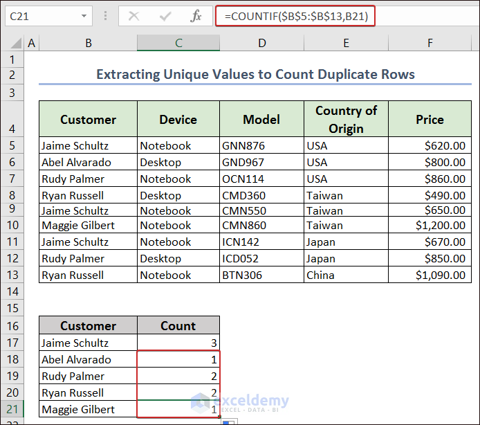
We have a dataset with customer names and product details. With the following formula in cell C17, we can count the duplicate rows based on the customer names considering the first occurrence.
=COUNTIF($B$5:$B$13,B17)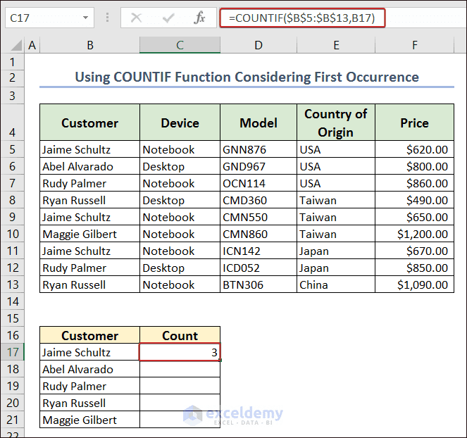
The COUNTIF function counts the duplicate rows in the range $B$5:$B$13 based on the value in cell B17.
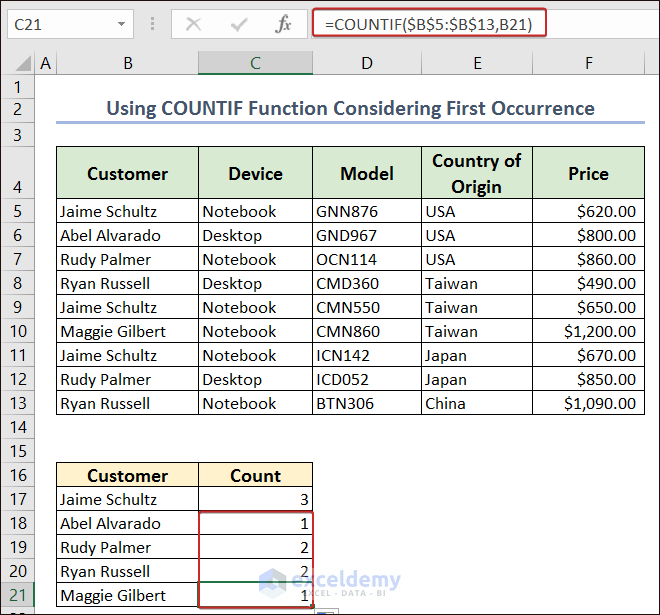
Use Fill Handle to AutoFill the other cells in column C to see the number of duplicate rows.
1.2 Count Duplicate Rows Ignoring First Occurrence
To count the duplicate rows based on customer names ignoring the first occurrence, apply the following formula in cell D17.
=COUNTIF($B$5:$B$13,B17)-1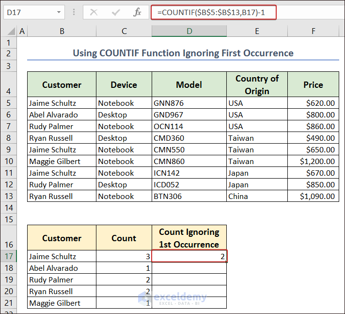
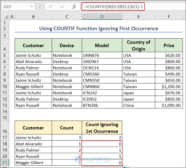
AutoFill the rest of the cells in column D with Fill Handle.
Read More: How to Count Duplicates in Column in Excel
Example 2 – Use COUNTIFS to Count Duplicate Rows for Multiple Conditions
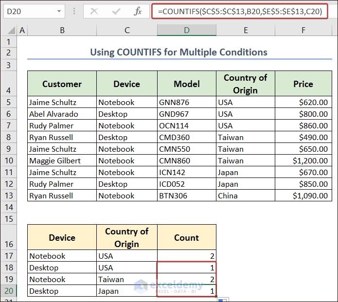
To count duplicate rows in the Device and Country of Origin columns, add the following formula in cell D17 and press Enter.
=COUNTIFS($C$5:$C$13,B17,$E$5:$E$13,C17)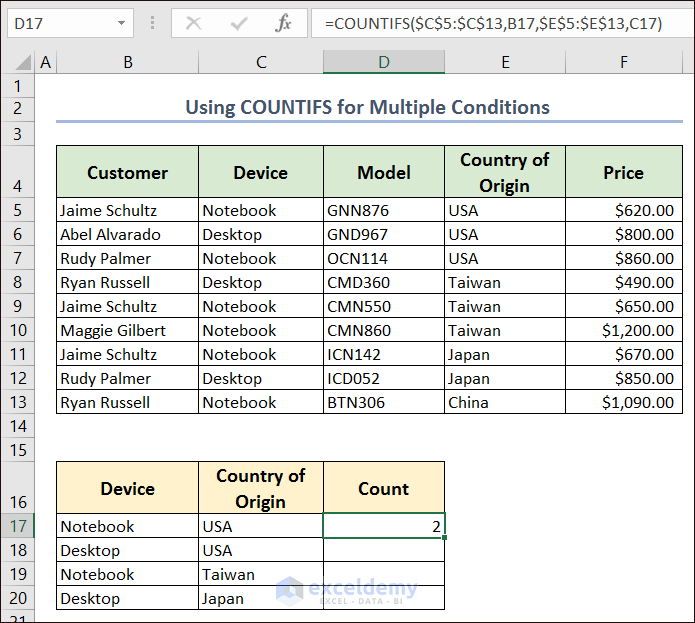
The COUNTIFS function considers the values in cells B17 and C17 and counts the duplicate rows that match in the range $B$5:$B$13 and $C$5:$C$13.
AutoFill the rest of the cells in column D with Fill Handle.
Read More: How to Count Duplicates in Two Columns in Excel
Example 3 – Count Total Duplicate Rows in Excel
3.1 Use IF and COUNTIF Functions
To find the duplicate rows based on the customer names, use the following formula.
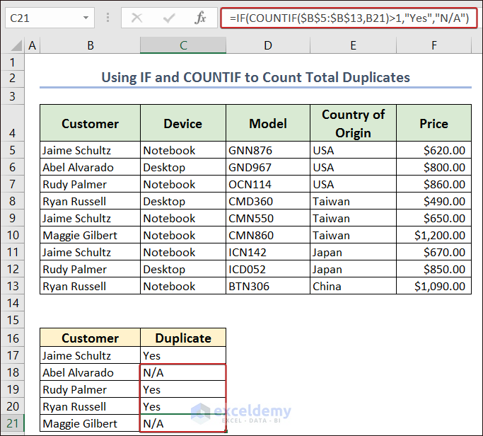
=IF(COUNTIF($B$5:$B$13,B17)>1,"Yes","N/A")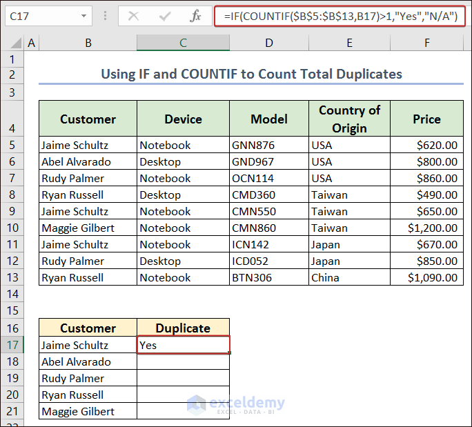
The COUNTIF function will count the number of matched cells in the range B5:B13 based on the value in cell B17. If the result gets more than 1, the output will be Yes as we have applied the IF function, otherwise it will output N/A.
AutoFill the other cells in column C.
Apply the following formula in cell C22 to get the total count of duplicate rows.
=COUNTIF(C17:C21,"Yes")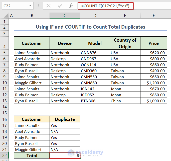
3.2 . Use COUNTIF with IF, SUM, and ROWS Functions
To get the total count of the duplicate rows in Excel, apply the following formula combining COUNTIF with IF, SUM, and ROWS functions.
=ROWS($B$5:$B$13)-SUM(IF(COUNTIF($B$5:$B$13,$B$5:$B$13) =1,1,0))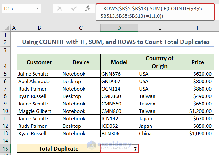
The ROWS function returns the total number of rows and the combination of the IF, SUM, and COUNTIF functions returns the total number of rows having no duplicate row.
Example 4 – Use SUM & EXACT Functions to Count Case Sensitive Duplicate Rows
We can count the duplicate rows based on the customer names by applying the following formula combination of the SUM and EXACT functions.
Note: The EXACT function is case sensitive.
=SUM(--EXACT($B$5:$B$13,B17))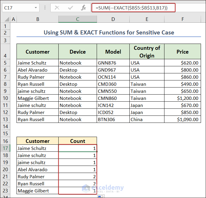
The EXACT function finds the exact match value in range B5:B13 considering the value in cell B17. The SUM function returns the summation of the number of duplicate rows.
Read More: How to Count Duplicate Values in Multiple Columns in Excel
Example 5 – Count Duplicate Rows by Extracting Unique Values with UNIQUE Function
We can ignore the duplicate values and find the unique values by using the UNIQUE function. Apply the following formula in cell B17 to extract the unique values.
=UNIQUE(B5:B13)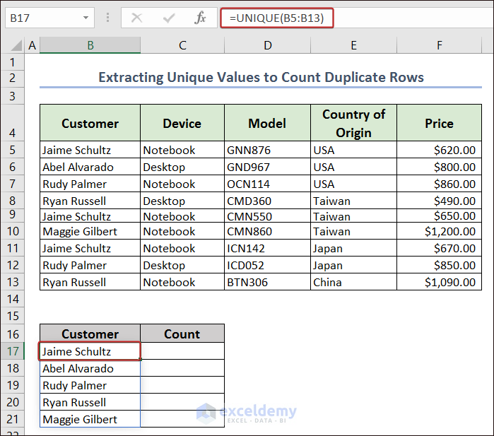
Based on the unique values, we can find the number of each value in a specific range with the COUNTIF function. Add the formula below in cell C17,
=COUNTIF($B$5:$B$13,B17)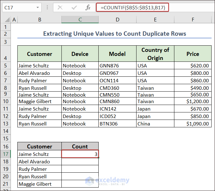
AutoFill the rest of the cells in column C with Fill Handle. It will display both the duplicate values and the duplicate rows.
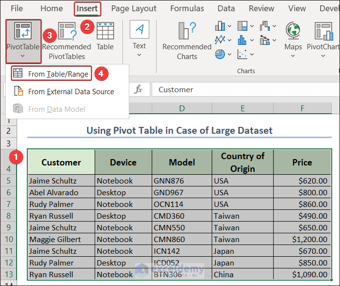
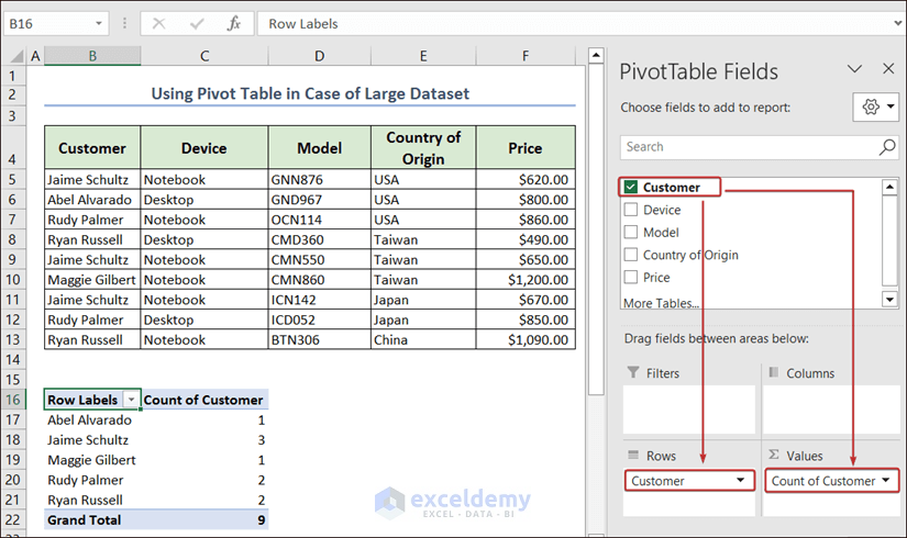
Example 6 – Use Pivot Table to Count Duplicate Rows in Case of Large Excel Dataset
For large datasets, we can use the Pivot Table to count the duplicate rows in Excel. For this, we need to create a Pivot Table first.
To create a Pivot Table,
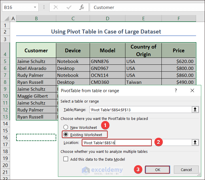
A wizard named PivotTable from table or range will appear.
Select the Existing Worksheet and define a cell (i.e. B16). Click on OK to insert the Pivot Table.
Drag the Customer option in the PivotTable Fields to the Rows and Values sections. We will get the Pivot Table in the defined location with the count of the duplicate rows.
How to Filter Duplicate Rows with Filter Feature in Excel
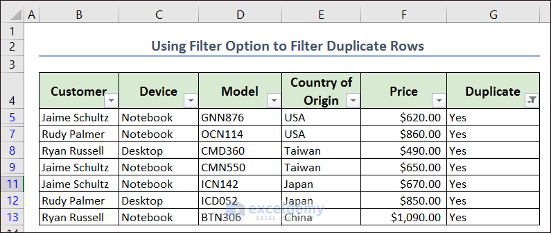
To filter duplicate rows with the help of the Filter feature, create a separate column G and apply the following formula in cell G5 to identify the duplicate rows.
=IF(COUNTIF($B$5:$B$13,B5)>1,"Yes","")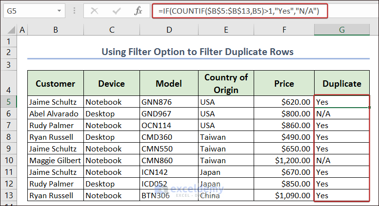
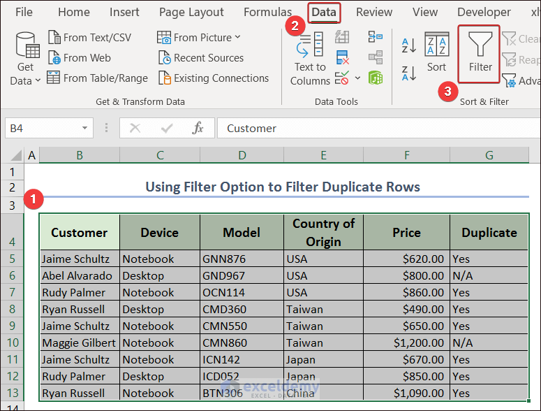
Select the entire dataset and click on Filter from the ribbon under Data.
Click on the arrow in the Duplicate column and select the Yes option. Click OK to finish the process.
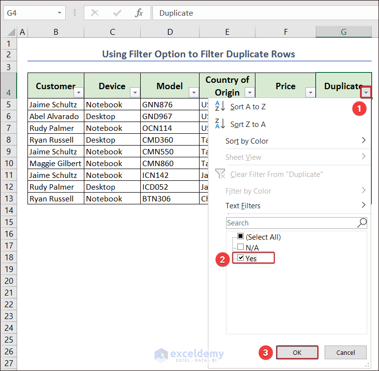
The duplicate rows will be filtered.
Frequently Asked Questions
1. How to select duplicates in Excel?
In order to select all the duplicates after filtering them, use the CTRL + A command.
2. How to clear or remove duplicates in Excel?
After filtering the duplicate rows, select all of them. Then, right-click on the mouse and select Delete rows from the available options to clear or remove duplicates in Excel.
3. How to highlight duplicates in Excel?
In order to highlight duplicates in Excel, select all the filtered duplicates. Go to the Home tab and select a color from Fill to highlight duplicates.
4. How to copy or move duplicates to another sheet?
Select all the filtered duplicate cells and press CTRL + C to copy them. Pick a cell in the destination sheet and press CTRL + V to copy or move the duplicates.
Download Practice Workbook
Related Articles
- Count Number of Occurrences of Each Value in a Column in Excel
- Count the Order of Occurrence of Duplicates in Excel
- How to Count Duplicates Based on Multiple Criteria in Excel
- How to Count Occurrences Per Day in Excel
<< Go Back to Duplicates in Excel | Learn Excel
Get FREE Advanced Excel Exercises with Solutions!

1. You could simplify the last formula, by removing the whole part about =ROWS(), using:
IF(COUNTIF($B$5:$B$10,$B$5:$B$10) =2,1,0).
All it took was to use “=2” instead of “=1”.
(Note. if your purpose was to explain the use of ROWS, then great).
2. What I am looking for is total COUNT of whole (or part) row duplicates.
eg. Liz and Apple, Joe and Apple, Joe and Orange (total of how many such rows are repeated) BUT – WITHOUT creating any new columns, which would be too easy. In your table above, the answer would be “1” because ONLY Liz and Apple is repeated. I assume this would require COUNTIFS, possibly an array. But can’t get it to work. Please let me know if you have anything on this. (Note. I often share links to your site, when I help friends in different countries with Excel)
Hi Alex, it is a great pleasure for us to know that you are getting benefits from our content (and referring us to your friends too)!
Now, your answers:
1. No, you have to use the ROWS function too. Otherwise, you will not get the correct answer in other cases (your guess is true only for this particular set of data).
2. Yes. You are right. You have to use the COUNTIFS function. Use the following formula.
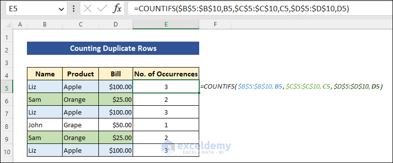
=COUNTIFS($B$5:$B$10,B5,$C$5:$C$10,C5,$D$5:$D$10,D5)If you have two columns only, remove the $D$5:$D$10,D5 part from the formula, i.e.
=COUNTIFS($B$5:$B$10,B5,$C$5:$C$10,C5)Now, copy the formula down. The output number will say how many times each row is repeated.
Regards
-Mahdy
(ExcelDemy Team)