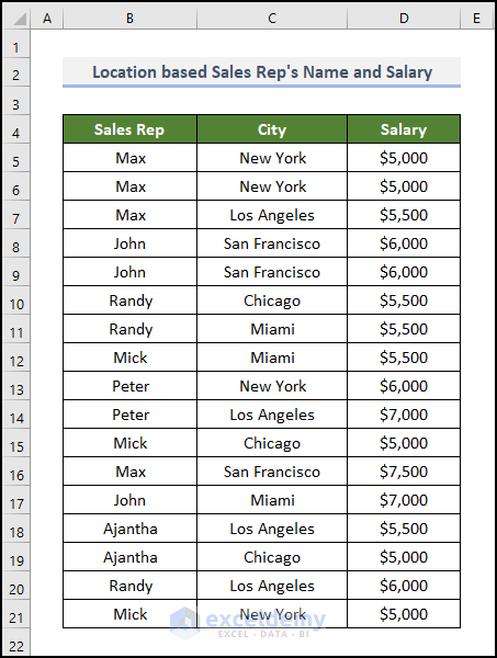
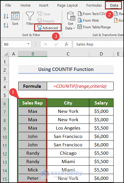
We have the Sales Rep, City, and Salary columns. There are a few values that are repeated within the columns. We’ll count the number of occurrences of each value in a column in multiple ways.
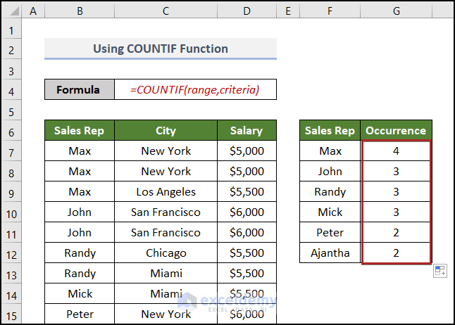
Method 1 – Using the COUNTIF Function
Steps:
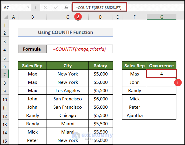
- Use the following formula in E7:
=COUNTIF(B7:B23,F7)
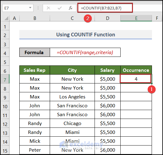
Within the COUNTIF function, we inserted all the values of Sales Rep as range. Our criteria were every name, since we need to calculate the number of instances for every name. So as criteria we have inserted a name (first name in this case, gradually will check using every other name). It gave the number of occurrences for the name Max. As our data set is not a big one, you can have a quick look and find there are 4 Max inside that Sales Rep column.
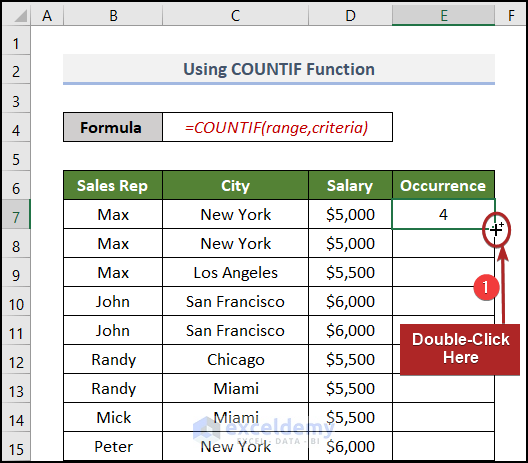
- Bring the cursor to the bottom-right corner of cell E7 and it’ll look like a plus (+) sign. It’s the Fill Handle tool.
- Double-click on it for the rest of the values.
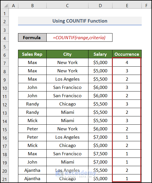
The formula doesn’t provide the correct values since the lookup range also moves when copying the formula.
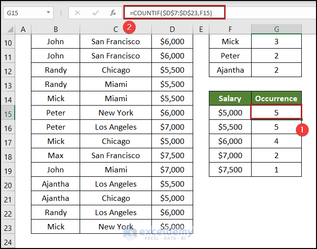
- Replace the formula with the following:
=COUNTIF($B$7:$B$23,F7)

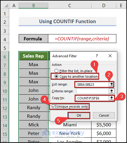
Let’s display the results solely on unique values:
- Select the whole Sales Rep column (B6:B23).
- Go to the Data tab.
- Select the Advanced option in the Sort & Filter group.
- Select Copy to another location.
- The List Range is automatically selected as we select if before.
- In the Copy to box, insert the cell reference where you want to paste it. In this case, we gave it as cell F6.
- Check the box for Unique records only.
- Hit Enter or click OK.
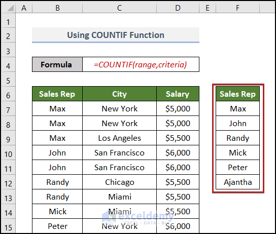
- We can see all the unique values from the column in a separate location in the F6:F12 range.
- Let’s use the previous COUNTIF formula.
- Use the AutoFill feature to copy the formula to the following cells.
- Here’s the formula for the Salary column of our example.
=COUNTIF($D$7:$D$23,F15)
Note: From here on, we will extract the unique values to separate locations using the Sort & Filter option before using any formula.
Read More: How to Count Duplicates in Column in Excel
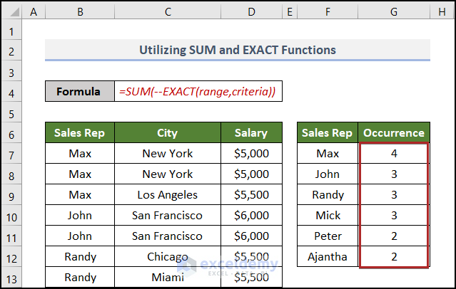
Method 2 – Utilizing SUM and EXACT Functions
Steps:
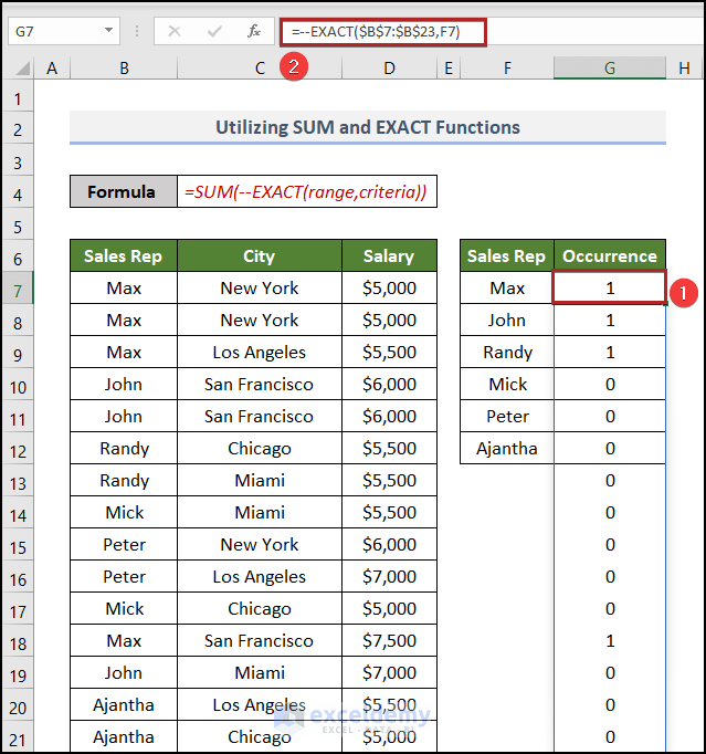
- Select cell G7 and enter the following formula.
=--EXACT($B$7:$B$23,F7)
We have written the EXACT function for Sales Rep. We used a double hyphen to convert TRUE/FALSE to 1 and 0.
- Wrap the formula in a SUM:
=SUM(--EXACT($B$7:$B$23,F7))
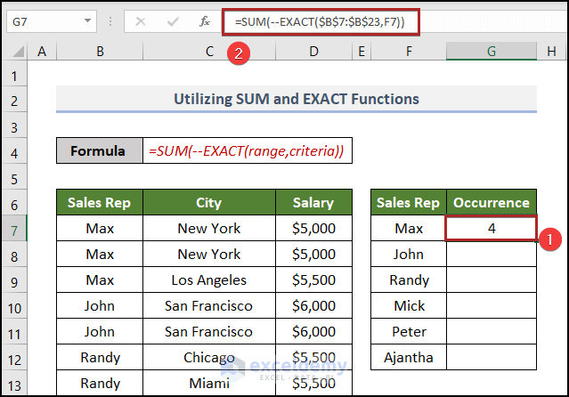
- Since this is an array formula, you need to use Ctrl + Shift + Enter instead of just ENTER to operate this formula. If you are using Excel 365, you apply it with Enter.
- Use the Fill Handle to copy the formula down.
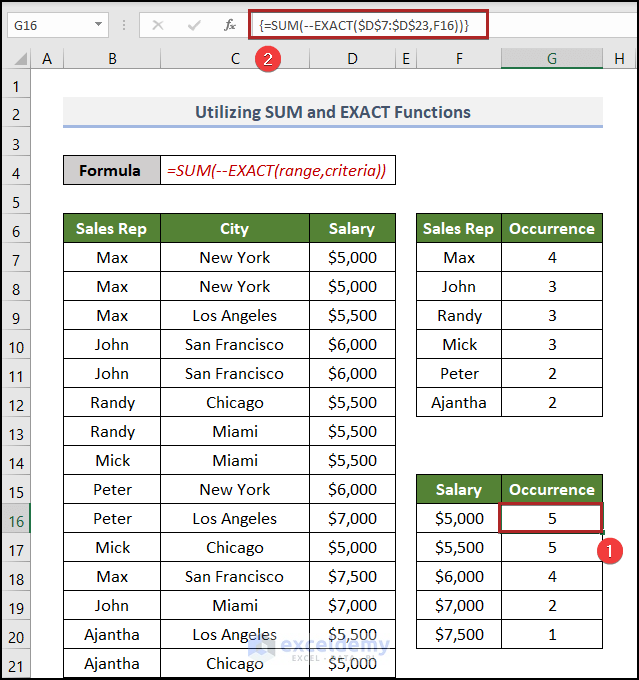
Similarly, you can use the formula for the numbers as well. Here’s the formula for the Salary column:
=SUM(--EXACT($D$7:$D$23,F16))
Read More: How to Count Duplicates in Two Columns in Excel
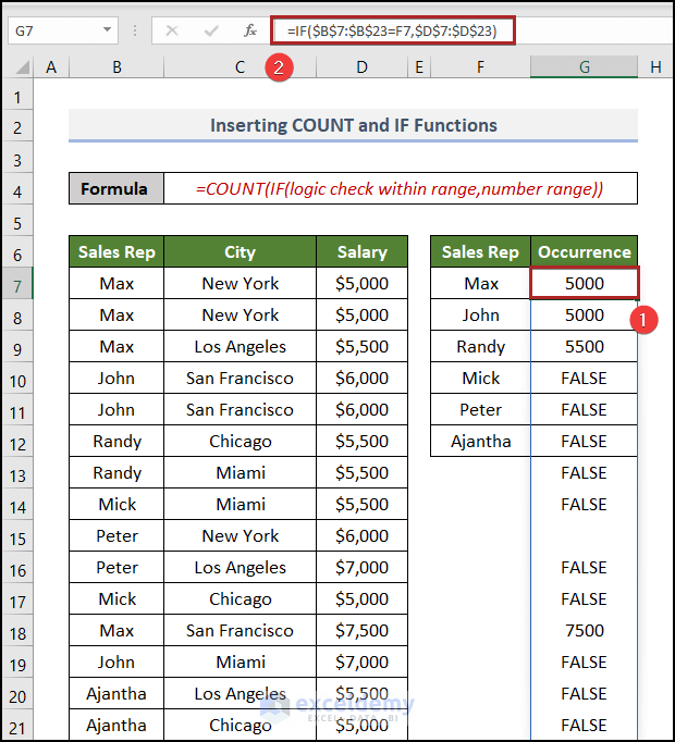
Method 3 – Inserting COUNT and IF Functions
Steps:
- Insert this formula in G7 for the Sales Rep column.
=IF($B$7:$B$23=F7,$D$7:$D$23)
- Press Enter.
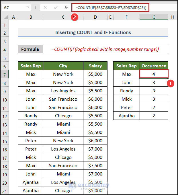
- Wrap the formula in COUNT so it becomes:
=COUNT(IF($B$7:$B$23=F7,$D$7:$D$23))
- You can do this for the number values. Replace the fields with the appropriate ranges and criteria.
=COUNT(IF($D$7:$D$23=F16,$D$7:$D$23))
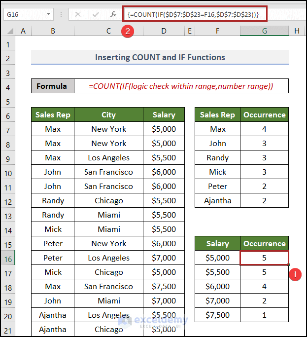
Note: Make sure your second parameter within the IF function is a number range and you are using Absolute Reference.
Read More: How to Count Duplicate Values in Multiple Columns in Excel
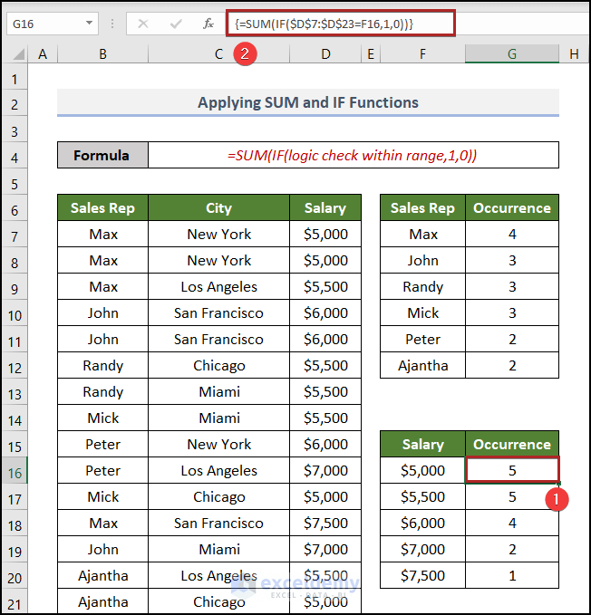
Method 4 – Applying SUM and IF Functions
Steps:
- Fo to cell G7 and insert the formula below.
=SUM(IF($B$7:$B$23=F7,1,0))
- Hit Enter.

The formula will work fine for the number values as well:
=SUM(IF($D$7:$D$23=F16,1,0))
Read More: How to Count Duplicate Rows in Excel
Method 5 – Using a PivotTable
Steps:
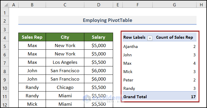
- Select any cell inside the range. Here, we selected cell B4.
- Go to the Insert tab.
- Click on PivotTable in the Tables group.

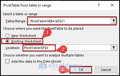
- The PivotTable from table or range dialog box will open.
- Check whether the Table/Range is correct.
- Select Exiting Worksheet as we want to insert the PivotTable in the same sheet.
- Provide the Location. We’ll put the table in cell F4.
- Click OK.
- The pivot table will appear.
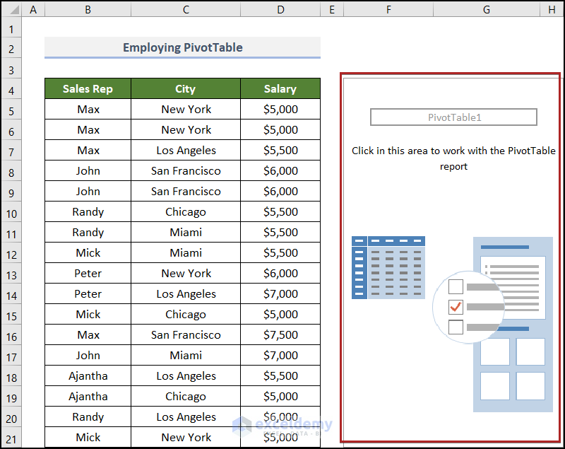
- Inside the PivotTable Fields task pane, you will see the table’s column name in the Field section and four areas: Filters, Columns, Rows, Values.
- Drag the Sales Rep field into the Rows and Values area.
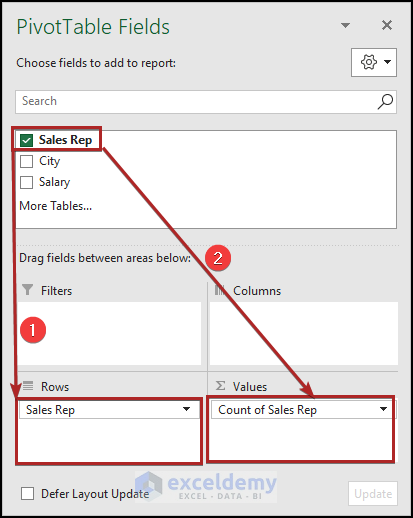
- It counts the occurrence number of each value within the Sales Rep column.
Read More: Count the Order of Occurrence of Duplicates in Excel
Counting Number of Occurrences with Multiple Criteria in Excel
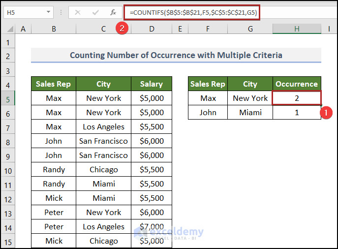
We’ll show the demo for Max and John. From the dataset, we can see that there are values for Max in New York, Los Angeles, and San Fransisco. We want to count Max just from New York city.
- Go to cell H5 and paste the following formula into the cell.
=COUNTIFS($B$5:$B$21,F5,$C$5:$C$21,G5)
Here, we used the COUNTIFS function which is able to take multiple criteria.
- Press Enter.
Download the Practice Workbook
Further Readings
- How to Count Duplicates Based on Multiple Criteria in Excel
- How to Count Occurrences Per Day in Excel
<< Go Back to Count Duplicates in Excel | Learn Excel
Get FREE Advanced Excel Exercises with Solutions!
