Method 1 – SUMPRODUCT Function to Count Duplicates Based on Multiple Criteria
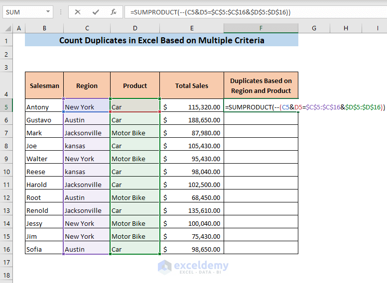
- Enter the following formula in cell F5,
=SUMPRODUCT(--(C5&D5=$C$5:$C$16&$D$5:$D$16))The formula will return 1 for each unique set of regions and products and will give the number of occurrences for duplicate sets of region and product.
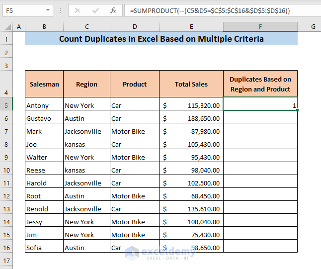
- Press ENTER,
It will give an output of 1. That means there is only one car seller in New York. There are no duplicates.
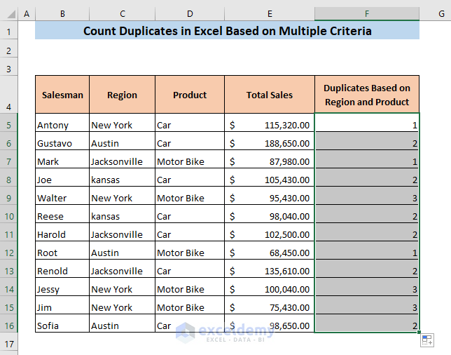
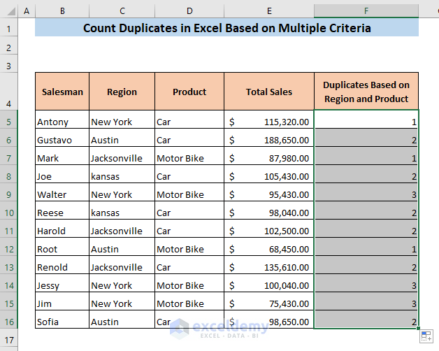
- Drag the fill handle from cell F5 to the end of your dataset.
You will get the count of the duplicates in your dataset based on multiple criteria which are sales region and product type.
Related Content: How to Count Duplicates in Column in Excel
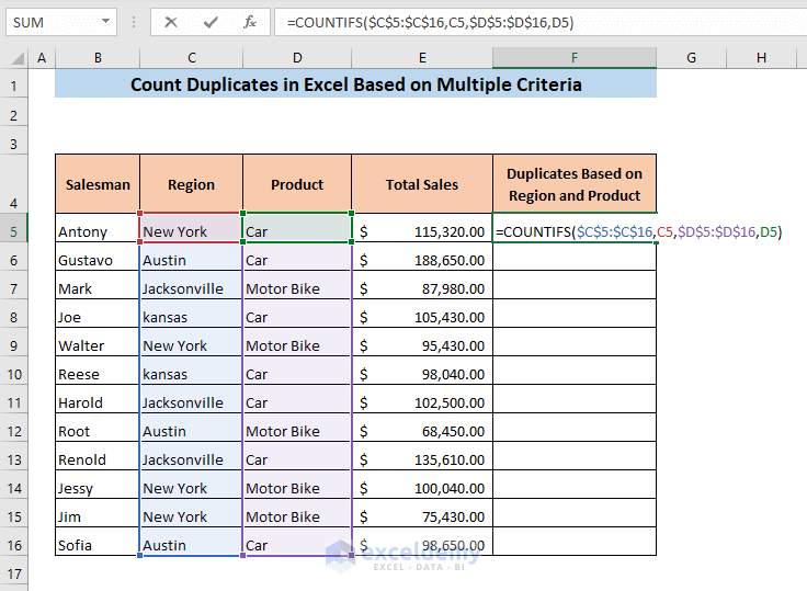
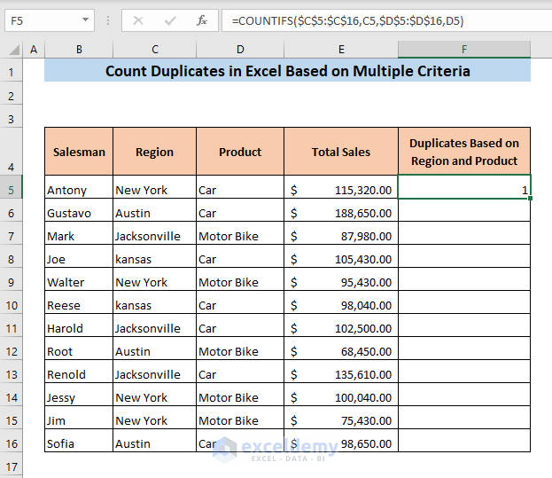
Method 2 – COUNTIFS Function to Count Duplicates Based on Criteria
- Enter the following formula in cell F5:
=COUNTIFS($C$5:$C$16,C5,$D$5:$D$16,D5)The formula will return 1 for each unique set of regions and products and will give the number of occurrences for duplicate sets of region and product.
- Press ENTER.
It will give an output of 1. That means there is only one car seller in New York. There are no duplicates.
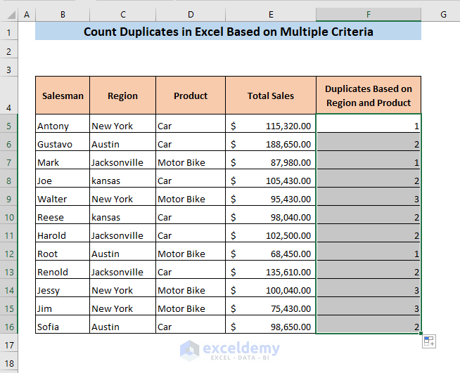
- Drag the fill handle of cell F5 to the end of your dataset.
You will get the count of the duplicates in your dataset based on multiple criteria.
Read More: How to Count Duplicates in Two Columns in Excel
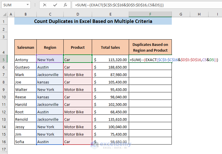
Method 3 – Count Duplicates Based on Multiple Criteria Using SUM and EXACT Functions
- Enter the following formula in cell F5:
=SUM(--(EXACT($C$5:$C$16&$D$5:$D$16,C5&D5)))The EXACT function gives TRUE, if it finds an exact match of product and region among the range. The double dash in the formula (—) converts the TRUE into 1. The SUM function adds up all the ones.
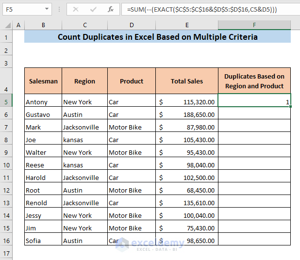
- Press ENTER.
It will give an output of 1. That means there is only one car seller in New York. There are no duplicates.
- Drag the fill handle from cell F5 to the end of your dataset.
You will get the count of the duplicates in your dataset based on multiple criteria which are sales region and product type.
Related Content: How to Count Duplicate Values in Multiple Columns in Excel
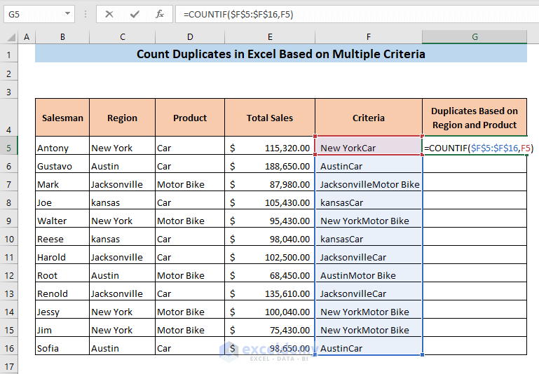
Method 4 – Count Duplicates by Combining Criteria Altogether
- Enter the following formula in cell F5:
=C5&D5It will combine the criteria from cells C5 and D5 in cell F5.
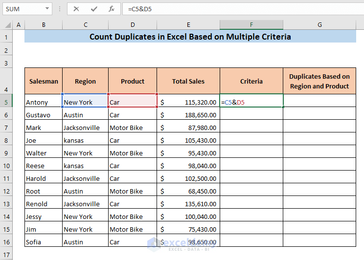
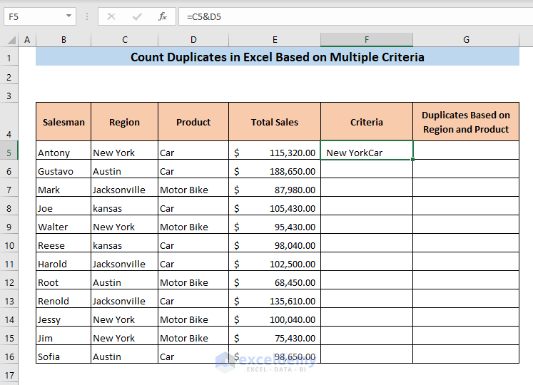
- Press ENTER.
You will get the combined criteria in cell F5.
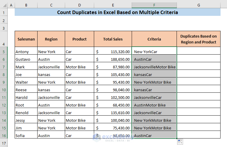
- Drag the fill handle in cell F5 to the end of your dataset.
You can use the COUNTIF function to count the duplicates.
- Enter the following formula in cell G5:
=COUNTIF($F$5:$F$16,F5)The formula will return 1 for unique values and the number of occurrences for duplicate values.
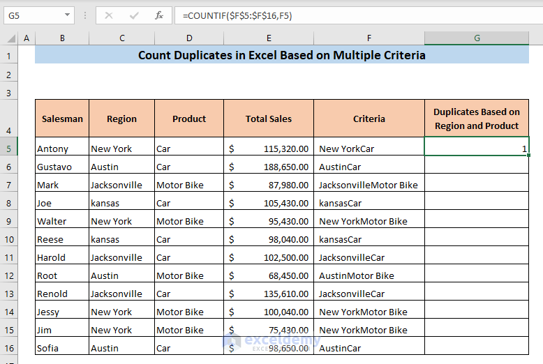
- Press ENTER.
It will give an output of 1. That means there is only one car seller in New York. There are no duplicates.
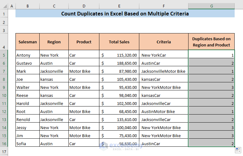
- Drag the fill handle of C5 to the end of your dataset.
You will get the count of the duplicates in your dataset based on multiple criteria which are sales region and product type.
Read More: How to Count Duplicate Rows in Excel
Download the Practice Workbook
Related Articles
- Count Number of Occurrences of Each Value in a Column in Excel
- Count the Order of Occurrence of Duplicates in Excel
- How to Count Occurrences Per Day in Excel
<< Go Back to Duplicates in Excel | Learn Excel
Get FREE Advanced Excel Exercises with Solutions!

Hi Prantick,
Would you know which of the 3 first methods takes less memory?
The 4th is already discarded because it uses 2 columns instead of one.
Thank you very much,
Thanks for your question, Jorge F. The allocation of memory mostly depends upon the dataset in which you are working on, and how they are interacting to other functions. For example, if you use a nested function, that function will cost more memory. There are some functions out there that consume more memory compared to other functions. Among the methods described above, the SUMPRODUCT function has more memory allocation compared to other functions. The other two methods would consume more or less the same amount of memory.