Looking for ways to use the COUNTIF function with conditional formatting in Excel? Then, this is the right place for you. We can highlight cells depending on different criteria using conditional formatting. For this purpose, you may use different formulas to select specific cells. Here, you will find 7 examples of using the COUNTIF function in those formulas to format cells in Excel.
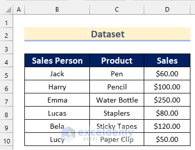
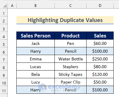
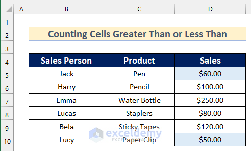
Here, we have a dataset containing the names of some Sales Person, Product, and their Sales values. Now, we will show how you can use the COUNTIF function with conditional formatting using this dataset in Excel.
1. Highlighting Duplicate Values Using COUNTIF Function with Conditional Formatting
Sometimes, you may have duplicate values in your dataset that you want to highlight. You can highlight these duplicate values using the COUNTIF function with conditional formatting in Excel.
Here are the steps.
Steps:
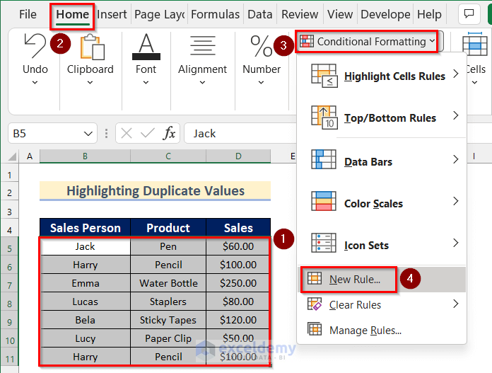
- Firstly, select cell range B5:D11.
- Then, go to the Home tab >> click on Conditional Formatting >> select New Rule.
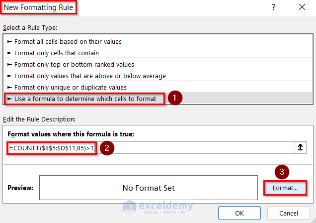
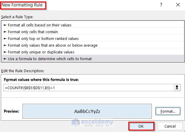
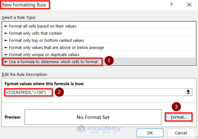
- Now, the New Formatting Rule box will appear.
- Next, select Use a formula to determine which cells to format.
- After that, insert the following formula in the box.
=COUNTIF($B$5:$D$11,B5)>1- Then, click on Format.
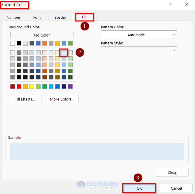
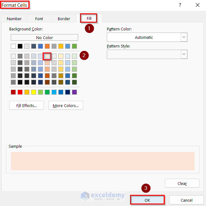
- Now, the Format Cells box will open. Using this box, you can format cells according to your wish.
- Here, we will go to the Fill option.
- Then, select Blue, Accent 5, Lighter 80% as Background Color.
- After that, click on OK.
- Again, the New Formatting Rule box will open.
- Lastly, click on OK.
- Finally, you will see that the duplicate cells have been highlighted.
Read More: How to Calculate Frequency Using COUNTIF Function in Excel
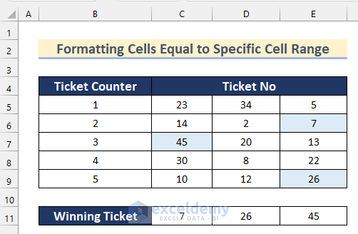
2. Applying COUNTIF Formula to Format Cells Equal to Specific Cell Range
Suppose, you have a dataset containing some Ticket No from 5 different Ticket Counters and also the Winning Ticket numbers in a different cell range. Now, if you want you can highlight the cells containing the winning ticket numbers in the dataset using the COUNTIF formula in conditional formatting.

Follow the steps given below to do that.
Steps:
- To start with, select cell range C5:E9.
- After that, go to the Home tab >> click on Conditional Formatting.
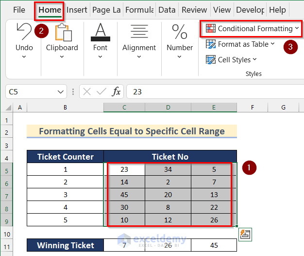
- Then, select New Rules.

- Now, the New Formatting Rule box will appear.
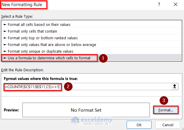
- Next, select Use a formula to determine which cells to format.
- Afterward, insert the following formula in the box.
=COUNTIF($C$11:$E$11,C5)>=1- Then, click on Format.
- After that, format the cells going through the same steps shown in Example 1.
- Thus, you will be able to format cells equal to a specific cell range by inserting the COUNTIF formula in conditional formatting.
Read More: COUNTIF Between Two Cell Values in Excel
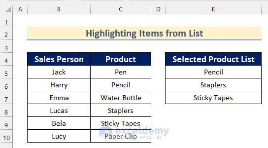
3. Highlighting Items from List Using Conditional Formatting in Excel
Next, we will show you how you can highlight items from a list or use a named range using conditional formatting in Excel.
Here, we have a dataset containing the names of some Sales Person and Product. Now, suppose you want to highlight the cells in the dataset that represent the Selected Product List.
Here are the steps that you need to follow to do this.
Steps:
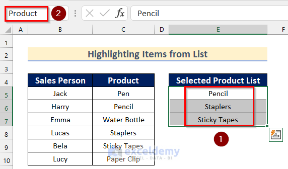
- Firstly, select cell range E5:E7.
- Then, go to the Name box and type “Product”.
- Next, press Enter.
- Now, select cell range C5:C10.
- After that, go to the Home tab >> click on Conditional Formatting >> select New Rules.

- Then, insert the following formula in the New Formatting Rule box.
=COUNTIF(Product,C5)- Afterward, click on Format.

- Lastly, format cells going through the same steps shown in Example 1.
- Thus, you can highlight items from a list using conditional formatting in Excel.

Read More: Excel COUNTIF to Count Cells Greater Than 1
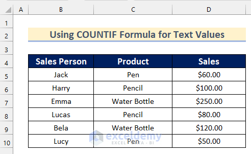
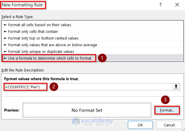
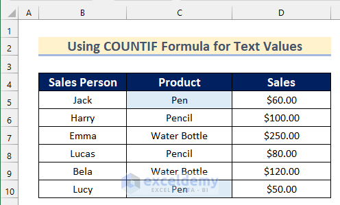
4. Utilizing Excel COUNTIF Formula for Text Values in Conditional Formatting
In the fourth example, we will show you how you can format cells that contain a specific text value by applying the COUNTIF formula in conditional formatting.
Follow the steps given below to do that.
Steps:
- In the beginning, select cell range C5:C10.
- Next, go to the Home tab >> click on Conditional Formatting >> select New Rule.

- Then, choose Use a formula to determine which cells to format as Rule type.
- Now, type the following formula in the box.
=COUNTIF(C5,"Pen")- Lastly, click on Format.
- After that, format the cells according to your choice as shown in Example 1.
- Finally, you will get the cells that contain that “Pen” as a text value by applying the COUNTIF function.
Read More: COUNTIF Function to Count Cells That Are Not Equal to Zero
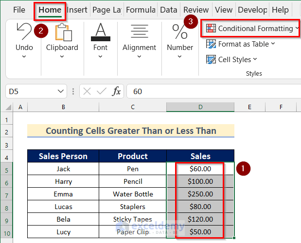
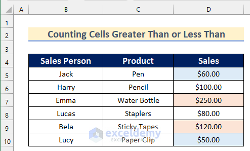
5. Counting Cells Greater Than or Less Than Using Conditional Formatting
If you want to highlight cells that contain greater than or less than a particular value, you can also do that using the COUNTIF formula in conditional formatting in Excel.
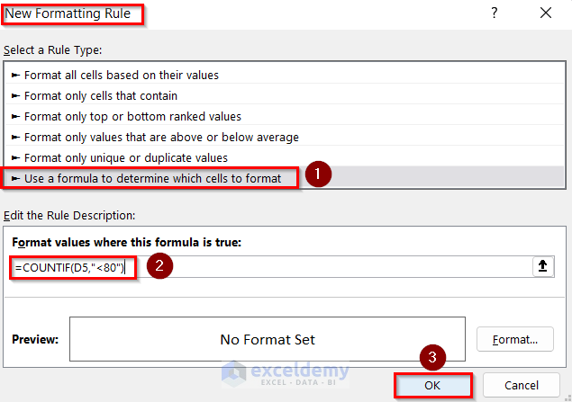
Here, we will show you how you can highlight cells that contain values greater than $100 and less than $80. Go through the steps given below to do that on your own.
Steps:
- Firstly, select cell range D5:D10.
- After that, go to the Home tab >> click on Conditional Formatting.
- Then, select the New Rule.

- Now, in the New Formatting Rule box insert the following formula.
=COUNTIF(D5,"<80")- Next, click on Format and format cells similar to the way shown in Example 1.
- Thus, the cells that contain values less than $80 will be highlighted.
- Again, open the New Formatting Rule box by going through the steps shown above and insert the following formula.
=COUNTIF(D5,">100")- Similarly, click on Format.
- Now, the Format Cells box will appear.
- Then, go to the Fill option >> select Orrange, Accent 2, Lighter 80%.
- Lastly, click on OK.
- Again, press OK.
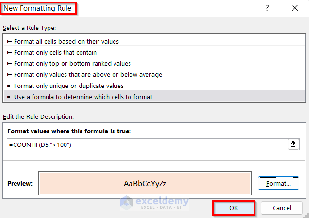
- Finally, the cells that contain values greater than $100 will be highlighted.
Read More: How to Use COUNTIF Function in Excel Greater Than Percentage
6. Applying the COUNTIF Function with Multiple Criteria for Conditional Formatting
Now, we will show you how you can apply the COUNTIF function with multiple criteria for conditional formatting in Excel.
Here, we will highlight the corresponding Sales Person’s name who had a Sales value less than $80 or greater than $120.
Steps:
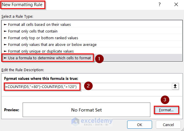
- To start with, open the New Formatting Rule box going through the same steps shown in Example 1.
- Then, type the following formula in the box.
=COUNTIF(D5,"<80")-COUNTIF(D5,">120")- Next, click on OK.
- Similarly, format the cells as shown in Example 1.
- Thus, you can use the COUNTIF function with multiple criteria for conditional formatting in Excel.

Read More: How to Use COUNTIF for Non Contiguous Range in Excel
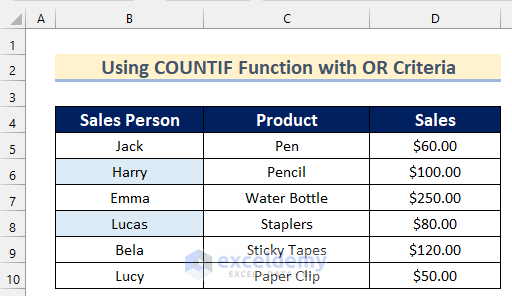
7. Formatting Cells Using Excel COUNTIF Function with OR Criteria
In the last example, you will find a way to format cells using the COUNTIF function with OR criteria in Excel.
Here, we will highlight the corresponding Sales Person’s name who sold Pencil and Staplers using conditional formatting.
Steps:
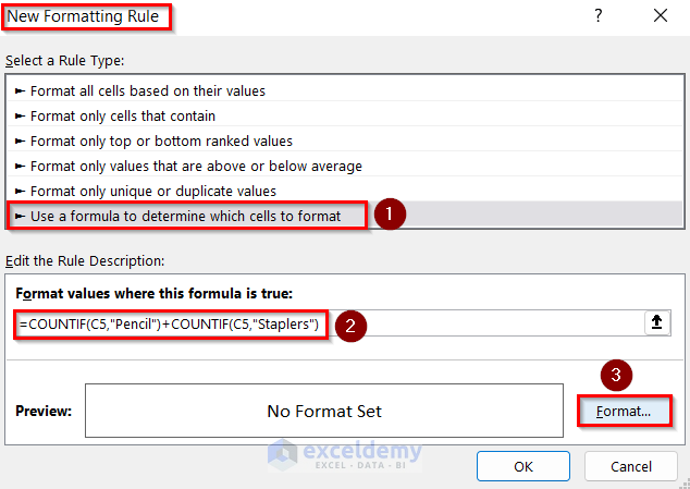
- Firstly, open the New Formatting Rule box going through the same steps shown in Example 1.
- Next, type the following formula in the box.
=COUNTIF(C5,"Pencil")+COUNTIF(C5,"Staplers")- After that, click on OK.
- Lastly, format cells going through the same steps shown in Example 1.
- Thus, you can format cells using the COUNTIF functions with OR criteria.
Read More: How to Compare Two Columns Using COUNTIF Function
Practice Section
In the article, you will find an Excel workbook like the image given below to practice on your own.

Download Practice Workbook
You can download the workbook to practice yourself.
Conclusion
So, in this article, we have shown you 7 examples of using the COUNTIF function with conditional formatting in Excel. I hope you found this article interesting and helpful. If something seems difficult to understand, please leave a comment. Please let us know if there are any more alternatives that we may have missed.
Related Articles
- How to Use COUNTIF Function to Calculate Percentage in Excel
- How to Use COUNTIF Function with Array Criteria in Excel
- How to Use Excel COUNTIF Between Time Range
- How to Use COUNTIF to Count Date Less Than Today in Excel
<< Go Back to Excel COUNTIF Function | Excel Functions | Learn Excel
Get FREE Advanced Excel Exercises with Solutions!
