We will use the following dataset of items and their quantities and grades to showcase how you can count duplicate items.
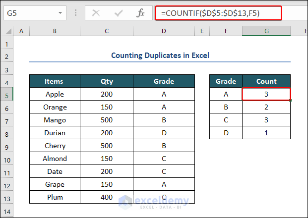
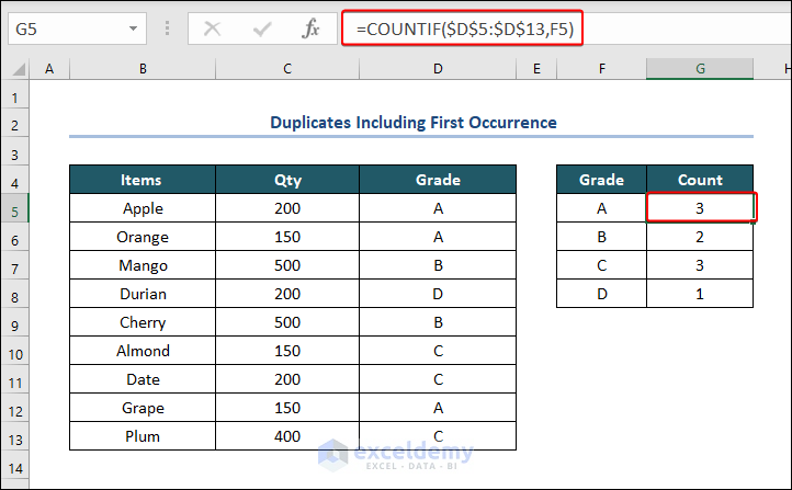
Method 1 – Using the COUNTIF Function to Count Duplicates in Excel (Including First Occurrence)
- Apply the following formula to count duplicates with the first occurrence in the Grade column.
=COUNTIF($D$5:$D$13,F5)- Use the Fill Handle to copy the formula for the cells below.
Method 2 – Inserting the COUNTIF Function for Counting Duplicates in Excel (Excluding the First Occurrence)
- Apply the following formula:
=COUNTIF($D$5:$D$13,F5)-1
Method 3 – Combining SUM and EXACT Functions to Count Case-Sensitive Duplicates
- Insert the following formula in a new cel:
=SUM(--EXACT($D$5:$D$13,F5))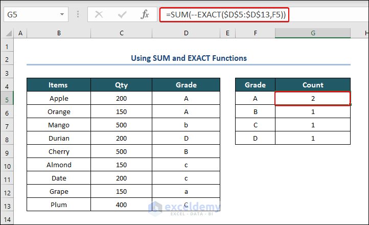
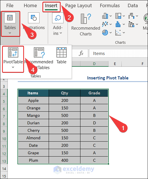
Method 4 – Inserting a Pivot Table to Count Duplicates in Excel
- Select the whole dataset.
- Go to Insert tab, select Tables, and choose Pivot Tables.
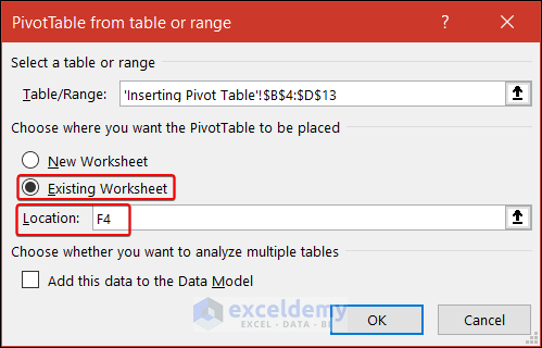
- In the dialog box, select Existing Worksheet and select the Range for pivot output if you want the pivot in the same worksheet.
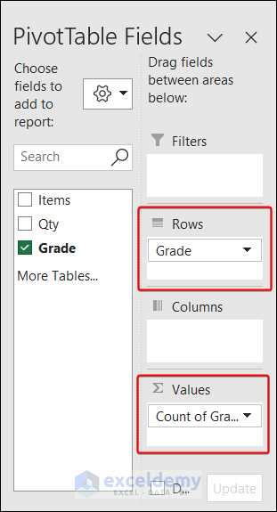
- In the Pivot Table Field from the right pane, put the Grade field in the Row and values sections.
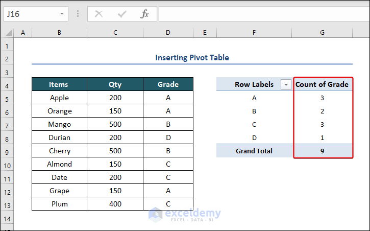
- You will see the pivot table counting the duplicates in the Grade column.
How to Count Duplicate Rows in Excel
- Apply the following formula.
=COUNTIFS($B$5:$B$13,B5,$C$5:$C$13,C5,$D$5:$D$13,D5)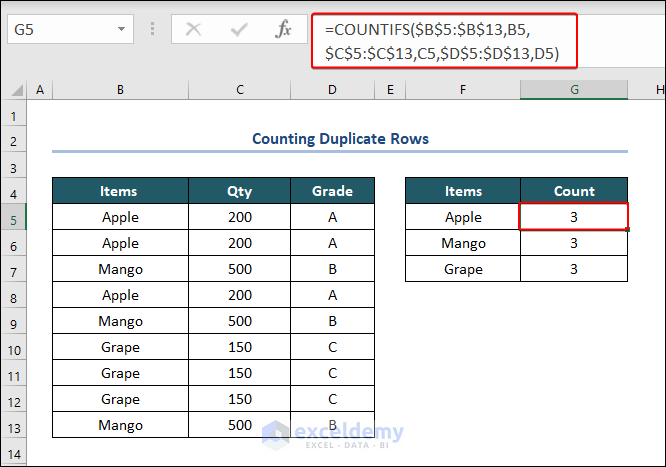
How to Count Duplicate Values with Multiple Criteria in Excel
We will count the duplicates in column Region using multiple conditions from columns Region and Product.
- Insert the following formula in a new cell.
=COUNTIFS($C$5:$C$13,C5,$D$5:$D$13,D5)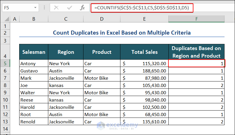
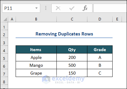
How to Remove Duplicates in Excel
- Select the dataset.
- Go to the Data tab, choose Data Tools, and select Remove Duplicates.
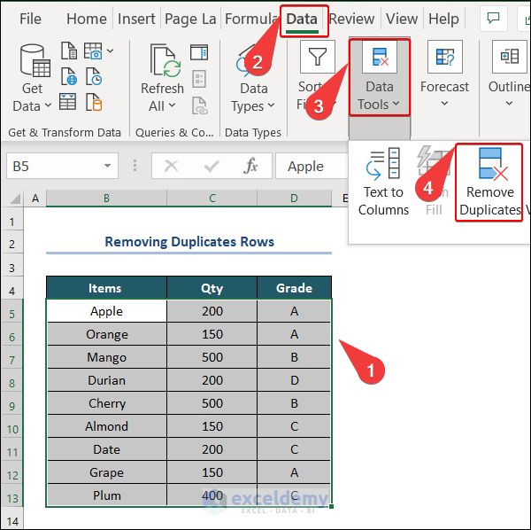
- We will get the duplicates removed.
Things to Remember
- Always use the “Absolute Cell Reference ($)” to “Block” the range
- While counting the case-sensitive duplicates, make sure to apply the formula as an “Array Formula” by Pressing “CTRL+SHIFT+ENTER”
- Use the unary operator (- -) to transform the result of the “EXACT” function to an array of 0 and 1’s.
Frequently Asked Questions
What does “Count Duplicates” mean in Excel?
“Count Duplicates” in Excel refers to the process of determining the number of occurrences or instances of duplicate values or entries within a column or range of cells in a worksheet.
Can I count duplicates based on multiple columns in Excel?
Yes, you can count duplicates based on multiple columns in Excel by combining criteria using formulas or PivotTables. For formulas, you can use the COUNTIFS function, which allows you to specify multiple conditions to count duplicates across different columns simultaneously.
Can I automate the process of counting duplicates in Excel using VBA?
Yes, you can automate the process of counting duplicates in Excel using VBA (Visual Basic for Applications). By writing a VBA macro, you can define custom logic to scan columns or ranges, count duplicates, and display or store the results in the desired format. This allows you to automate the duplicate counting process and apply it to multiple worksheets or workbooks efficiently.
Download the Practice Workbook
Count Duplicates in Excel: Knowledge Hub
- Excel Count Duplicates in Column
- Count Duplicates in Two Columns in Excel
- Count Duplicate Values in Multiple Columns in Excel
- Count Duplicate Rows in Excel
- Count Number of Occurrences of Each Value in a Column in Excel
- Count the Order of Occurrence of Duplicates in Excel
- Count Duplicates Based on Multiple Criteria in Excel
- Count Occurrences Per Day in Excel
- Ignore Blanks and Count Duplicates in Excel
- Use COUNTIF Formula to Find Duplicates
- Count Duplicate Values Only Once in Excel
- How to Count Repeated Words in Excel
- Count Duplicates with Pivot Table in Excel
- Excel VBA Count Duplicates in Range
- Excel VBA Count Duplicates in Column
<< Go Back to Learn Excel
Get FREE Advanced Excel Exercises with Solutions!
